Chapter 8 Nonlinear regression
In nonlinear regression we model an association where the response is not a linear function of the explanatory variable. Before considering nonlinear regression, it is always worth considering whether linear regression methods can be adapted, in either of two ways:
- Transform the explanatory and/or the response variable.
- Add additional functions (such as powers) of the explanatory variable, and perform multiple linear regression, the topic we examine in the following section.
The advantages of linear regression are that it is easier to do, more robust to fitting problems, and more widely available in statistical software. However, sometimes there are good reasons to fit a nonlinear function, or model, directly. The following examples show how to do this in R. They involve the nls function instead of lm.
Fitting nonlinear curves requires having a feel for the form of the mathematical formula you are using. We consider here the two most common nonlinear shapes, exponential and sigmoid.
8.1 Exponential curves
Exponential relationships are frequently seen in e.g. the biological sciences, where they arise in situations where the rate of change in some variable \(Y\) is a linear function of itself. An example of this would be the growth of a colony of bacteria in some medium. Initially, the number of bacteria in each new generation would be proportional to the number in the preceding generation, and the colony will grow exponentially.
The standard exponential is defined by the relationship \(Y = A + BR^X\). We have to estimate the three parameters \(A\), \(B\) and \(R\). The standard exponential is either continuously decreasing or increasing, and will be approximately either concave or convex everywhere in its range. When \(X = 0\), \(R^X = 1\) and therefore \(Y=A + B\); as \(X \rightarrow \infty\), \(Y\) either tends to an asymptote at \(A\) (if \(0 < R < 1\)) or tends to \(\pm\infty\) (if \(R > 1\)). The shape of the curve depends on the values taken by \(B\) and \(R\). The four possible scenarios are illustrated in the following figure showing some standard exponential curves of the form \(Y = A + BR^X\) with \(A=2\).
x <- seq(-6,+6,.1)

curve(2+5*1.5^x, col='black',xlim=c(-6,6),ylim=c(-25,+25), ylab="Exponential Curve" )
curve(2+5*0.5^x, col='green',xlim=c(-6,6), ylim=c(-25,+25), add=TRUE )
curve(2-5*0.5^x, col='red',  xlim=c(-6,6), ylim=c(-25,+25), add=TRUE )
curve(2-5*1.5^x, col='blue', xlim=c(-6,6), ylim=c(-25,+25), add=TRUE )
We will illustrate the use of the standard exponential using data from file frog.txt. Observations describe the electrical current flowing through the end-plate membrane of a frog’s muscle fibre following a jump in voltage. We wish to examine how the current changes with time.
frog <- read.table("frog.txt", header=TRUE)
with(frog, plot(Time, Current, pch=20, col='blue', ylim=c(0,90)))
These data exhibit the characteristic shape of an exponential curve with \(R < 1\) and \(B > 0\). We can assess the suitability of the standard curve by guessing the asymptotic value \(A\) (\(\approx 10\)), subtracting it from the \(Y\) values, taking logarithms of the results and then plotting these values against Time. If the standard model is appropriate, the result should be a straight line.
The linear nature of this plot suggests that the standard exponential is a reasonable function to try. We correspondingly fit the model \(Y=A+BR^X+\epsilon\).
We can use the nls function for this, but it often requires starting values for the parameter estimates. Otherwise it will choose 1.0 by default, but it might not work and then we need to make some guesses. Using the following specifications will work here.
Formula: Current ~ A + B * R^Time

Parameters:
   Estimate Std. Error t value Pr(>|t|)
A 1.114e+01  1.209e-01    92.1   <2e-16 ***
B 7.745e+01  3.005e-01   257.7   <2e-16 ***
R 8.709e-01  9.569e-04   910.2   <2e-16 ***
---
Signif. codes:  0 '***' 0.001 '**' 0.01 '*' 0.05 '.' 0.1 ' ' 1

Residual standard error: 0.5834 on 121 degrees of freedom

Number of iterations to convergence: 9
Achieved convergence tolerance: 2.294e-08
We use the parameter estimates to plot the estimated curve along with the observed data.
with(frog, plot(Time,Current, pch=20, col='blue', ylim=c(0,90)))
curve(11.14 + 77.45*0.8709^x, 0, 32, add=TRUE, lwd=2)
Confidence intervals for the parameter estimates are easy to obtain.
        2.5%      97.5%
A 10.8923104 11.3784054
B 76.8511431 78.0505008
R  0.8689657  0.8728412
Diagnostic plots should always be examined, but these are not so conveniently obtained as in linear regression. Some manual computing can be use instead.
resids <- residuals(m.frog.1)
fitted <- fitted(m.frog.1)
par(mfrow=c(1,2))
qqnorm(resids, main="Current ~ A+B*R^Time")
plot(fitted, resids, main=expression(Current ~ A+B*R^Time))
The q-q plot looks good so the residuals overall are approximately normally distributed. However, there is clearly systematic deviation from the fitted model. When the fit of the data to the model is good as in this case (a very small residual sum of squares), it might be not worth the extra work finding out the cause of the systematic deviations.
Prediction using predict with nls models provides point estimates but not confidence intervals.
[1] 29.28109 15.62941 11.155318.2 Sigmoid curves
These are S shaped curves, most frequently use for growth models. They are monotonic (either increasing or decreasing) and approach asymptotes at both extremes of \(X\). They will have a single point of inflexion, and hence will be concave in one section of their range and convex in the other. In general it is difficult to fit sigmoid curves accurately unless the full range of the curve (from lower asymptote to upper asymptote) is present in the data. An example would be the growth of bacteria in a closed medium. The population would initially grow exponentially, but as numbers became larger, the growth rate would increasingly become subject to constraints due to lack of resources. These constraints would become increasingly strong as the population grew larger, causing the growth rate to consistently decrease, and hence causing the population size to reach a plateau.
The logistic function defined by the relationship
\[Y=A+\frac{C}{1+e^{-B(X-M)}}\] specifies a symmetric sigmoid curve with a left-hand asymptote taking the value \(A\), a right-hand asymptote taking the value \(A+C\), and a central point of inflexion at \(X=M\), \(Y=A+\frac{C}{2}\), while the parameter \(B\) controls the rate at which the function moves between the two asymptotes: the greater \(B\) the steeper the slope. The following figure shows a standard logistic curve with parameters \(A=5, C=45, B=2\) and \(M=4\).
x <- seq(0,8,.5); A=5; C=45; B=2; M=4
y <- A+C/(1+exp(-B*(x-M)))
plot(x,y,col="blue", ylim=c(0,55))
lines(x,y,col="blue") # add line segments to join the points
abline(h=c(A,A+C),col="red", lty= "dashed")# add asymptotes
#next, indicate the point of inflection
lines(x=c(-1,M), y=c(A+C/2,A+C/2), col="green", lty="dashed")
lines(x=c(M,M), y=c(A+C/2,-1), col="green", lty="dashed")
# Add point and label at inflexion point
points(M,(A+C/2), pch=4,cex=2.5,lwd=3)
text(M+1,(A+C/2), "(M, A+C/2)")
The generalized logistic (or Richard’s) function is defined by the relationship
\[Y=A+\frac{C}{(1+Te^{-B(X-M)})^{\frac{1}{T}}}\] This function specifies a five parameter asymmetric sigmoid curve. The parameters \(A, B, C\) and \(M\) have the same interpretations as for the logistic curve, but the parameter \(T\), sometimes called the power law parameter, now specifies the value taken by the curve at the point of inflection, namely \(Y=A+C/(1+T)^{1/T}\). The asymmetry allowable in this sigmoid because of the parameter \(T\) provides greater flexibility in fitting to the data.
The Gompertz function is specified by the relationship
\[Y=A+Ce^{-e^{-B(M-X)}}\] and defines a limiting case of the generalized logistic which occurs when \(T\approx 0\). It is still asymmetric. The point of inflexion occurs at the point \(X=M\) and the asymptotes are \(A\) and \(A+C\).
These curves may be fitted to growth data of an ox (ox.txt). We plot the weight of the oxen against age. Fitting a logistic function here we can expect problems since the left-hand asymptote is not clearly visible in the dataset.
[1] "Age" "Weight" "Wtgain" "Intake"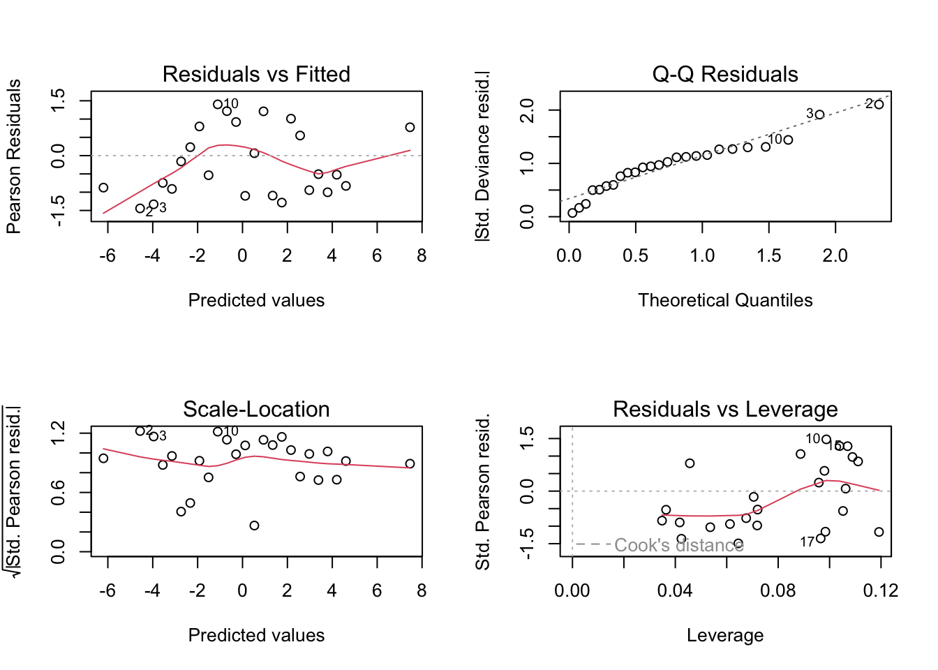
Fitting the logistic function:
m.ox.1 <- nls(Weight ~ A+C/(1+exp(-B*(Age-M))), start=list(A=0,C=600,M=50,B=0.05), data=ox)
summary(m.ox.1)
Formula: Weight ~ A + C/(1 + exp(-B * (Age - M)))

Parameters:
    Estimate Std. Error t value Pr(>|t|)
A -2.062e+02  3.876e+01  -5.319 9.69e-07 ***
C  8.761e+02  4.078e+01  21.485  < 2e-16 ***
M  3.254e+01  2.627e+00  12.388  < 2e-16 ***
B  3.392e-02  1.229e-03  27.593  < 2e-16 ***
---
Signif. codes:  0 '***' 0.001 '**' 0.01 '*' 0.05 '.' 0.1 ' ' 1

Residual standard error: 8.717 on 78 degrees of freedom

Number of iterations to convergence: 6
Achieved convergence tolerance: 2.551e-06 2.5% 97.5%
A -295.03832643 -139.67276798
C 805.80049610 969.33589792
M 26.70641214 37.14847947
B 0.03148137 0.03636619Note the very wide confidence interval for each asymptote.
For the generalized logistic:
m.ox.2 <- nls(Weight ~ A+C/(1+T*exp(-B*(Age-M)))**(1/T),
                start = list(A=0,C=600,M=50,B=0.05,T=0.1),
                data=ox)
summary(m.ox.2)
Formula: Weight ~ A + C/(1 + T * exp(-B * (Age - M)))^(1/T)

Parameters:
    Estimate Std. Error t value Pr(>|t|)
A  98.874368  13.432389   7.361 1.71e-10 ***
C 579.761193  12.382622  46.821  < 2e-16 ***
M  34.608067   1.325594  26.108  < 2e-16 ***
B   0.027535   0.001247  22.086  < 2e-16 ***
T  -0.501122   0.097073  -5.162 1.85e-06 ***
---
Signif. codes:  0 '***' 0.001 '**' 0.01 '*' 0.05 '.' 0.1 ' ' 1

Residual standard error: 8.02 on 77 degrees of freedom

Number of iterations to convergence: 7
Achieved convergence tolerance: 7.11e-06
We plot ox weight as a function of age with the generalized logistic curve.
with(ox, plot(Age,Weight,col="blue"))
curve(98.9 + 579.8/(1 -0.5 * exp(-0.0275 * (x - 34.6)))^(1/(-
0.5)),0,170,add=TRUE)
8.3 Non-parametric curve fitting
We can also fit smooth curves without specifying a mathematical form for them. Plot the data in lact.txt. Its shape does not conform to either the logistic or exponential form. We want to relate milk yield with days birth.
The first two data points are not bad values but are exactly what was expected in this study. It is possible to generate a best-fitting smooth spline through the data points and use this fitted curve to predict milk yield for any new value of day.
From https://www.stat.berkeley.edu/~s133/Smooth1a.html:
Spline smoothing, named after a tool formerly used by draftsmen. A spline is a flexible piece of metal (usually lead) which could be used as a guide for drawing smooth curves. A set of points (known as knots) would be selected, and the spline would be held down at a particular x,y point, then bent to go through the next point, and so on. Due to the flexibility of the metal, this process would result in a smooth curve through the points
With statistical curve fitting knot points are chosen and a cubic curve fitted through all the data points between each consecutive pair of knot points, in such a way as to ensure smoothness at the joins. The smoothing parameter, spar, in effect determines how many knot points are to be chosen.
spar = 0implies no smoothing, so a curve is fitted to every consecutive pair of points.spar = 1implies maximum smoothing, so a single cubic curve (i.e. a cubic regression) is fitted to the entire data set.
A drawback of this type of curve-fitting is that it does not provide a mathematical model and therefore we do not have parameters to help with interpretation.
The following code fits a smooth spline to the data and plots milk yield vs days after birth. To see the effect of increasing the amount of smoothing we consider spar = 0.4 (blue curve) and spar = 0.8 (green curve).
smsp4 <- with(lact, smooth.spline(Day, Yield, spar=0.4))
smsp8 <- with(lact,smooth.spline(Day,Yield, spar=0.8))
fitted4 <- fitted(smsp4)  # extract the fitted values
fitted8 <- fitted(smsp8)
with(lact,plot(Day,Yield))
points(lact$Day, fitted4, type="l", col="blue")
points(lact$Day, fitted8,type="l",col="green")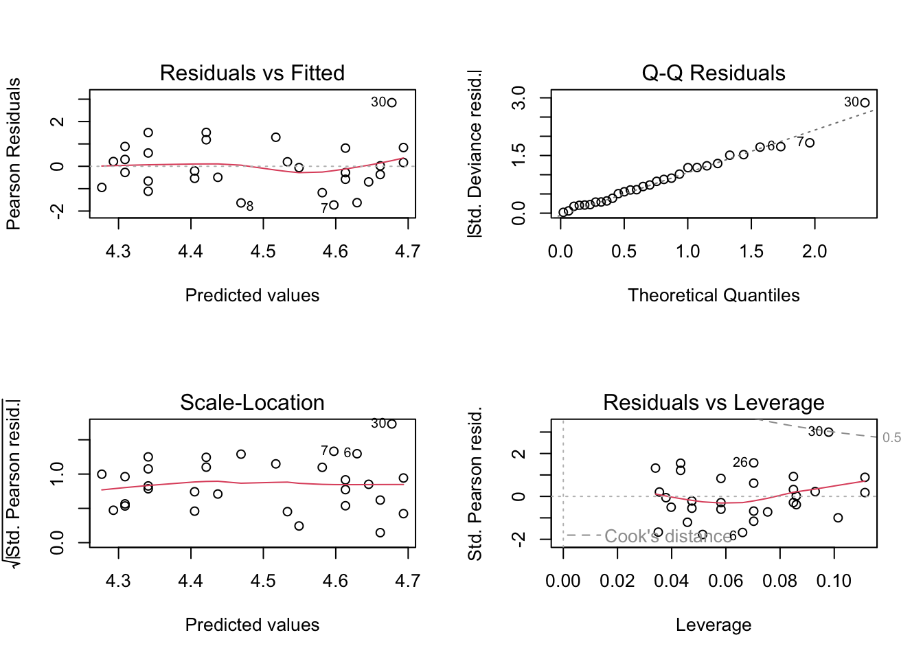
Note that we can predict from a smooth spline without having to put the new data into a data.frame, as we did for nls and lm models. Using the model fitted with spar = 0.4 we predict milk yields at 5 new days (predicted values plotted in red):
$x
[1]  50 100 150 200 250

$y
[1] 27.777126 22.663919 19.752909 21.145033  6.663466
8.4 Transforming the response variable
Sometimes it is appropriate to transform the response variable \(Y\) to achieve a linear model. We have already seen the log transformation:
\[\ln Y=a+bX+\epsilon\] Simple transformations of this type are legitimate provided the resulting residuals satisfy the necessary assumptions regarding normality, independence and equal variance at all values of \(X\). Apart from the log for continuous data or the square root, a well known transformation is the logit, used when the data are proportions or percentages, such that the \(Y\) values lie in the range \([0,1]\) or \([0,100]\). Denoting the proportions by \(p_i\), the definition is
\[\mbox{logit}(p_i)=\log\bigg(\frac{p_i}{1-p_i}\bigg)\] Note that the logit transformation is only defined for values of \(p_i\) in \((0,1)\); that is, values at the extremes are not allowed.
# create a sequence of values in [0.01, 0.99] in steps of 0.01
p <- seq(0.01,0.99,0.01)
logit <- log(p/(1-p))         # derive the logits of p
plot(p,logit,type="l",ylab="log(p/(1-p))")
Logits stretch the response values at the extremes, that is near zero and 1, where interest often lies and small differences really matter. The use of logits for proportion data does not guarantee that the residuals will have the desired properties.
We illustrate with data on the age of menarche for a sample of girls. Each girl was asked the date of her first period and the results grouped by age. Within each age group we have the total number of girls (Total), the number who had their first period (Menarche) and the mid-point of the age range for that group (Age).
    Age Total Menarche
1  9.21   376        0
2 10.21   200        0
3 10.58    93        0
4 10.83   120        2
5 11.08    90        2
6 11.33    88        5
We force the proportion into \((0,1)\) in this example by simply adding a small positive amount for illustration.
menarche$prop <- with(menarche, (Menarche+0.5)/(Total))
menarche$logitp <- with(menarche, log(prop/(1-prop)))
Warning in log(prop/(1 - prop)): NaNs produced
It looks like a linear model might be a sensible option to fit the transformed data.

Call:
lm(formula = logitp ~ Age, data = menarche)

Residuals:
     Min       1Q   Median       3Q      Max
-1.03525 -0.19546  0.04525  0.35859  0.53490

Coefficients:
             Estimate Std. Error t value Pr(>|t|)
(Intercept) -22.54265    0.63851  -35.30   <2e-16 ***
Age           1.72272    0.04897   35.18   <2e-16 ***
---
Signif. codes:  0 '***' 0.001 '**' 0.01 '*' 0.05 '.' 0.1 ' ' 1

Residual standard error: 0.4331 on 22 degrees of freedom
  (1 observation deleted due to missingness)
Multiple R-squared:  0.9825,    Adjusted R-squared:  0.9817
F-statistic:  1238 on 1 and 22 DF,  p-value: < 2.2e-16
While this analysis looks reasonable at first sight the diagnostic plots (see below) show that there is some room for improvement.
oldpar <- par()
# Modify them to do a 2x2 matrix of graphs
par(oma = c(0, 0, 0, 0), mfrow=c(2, 2))
plot(m.men.1)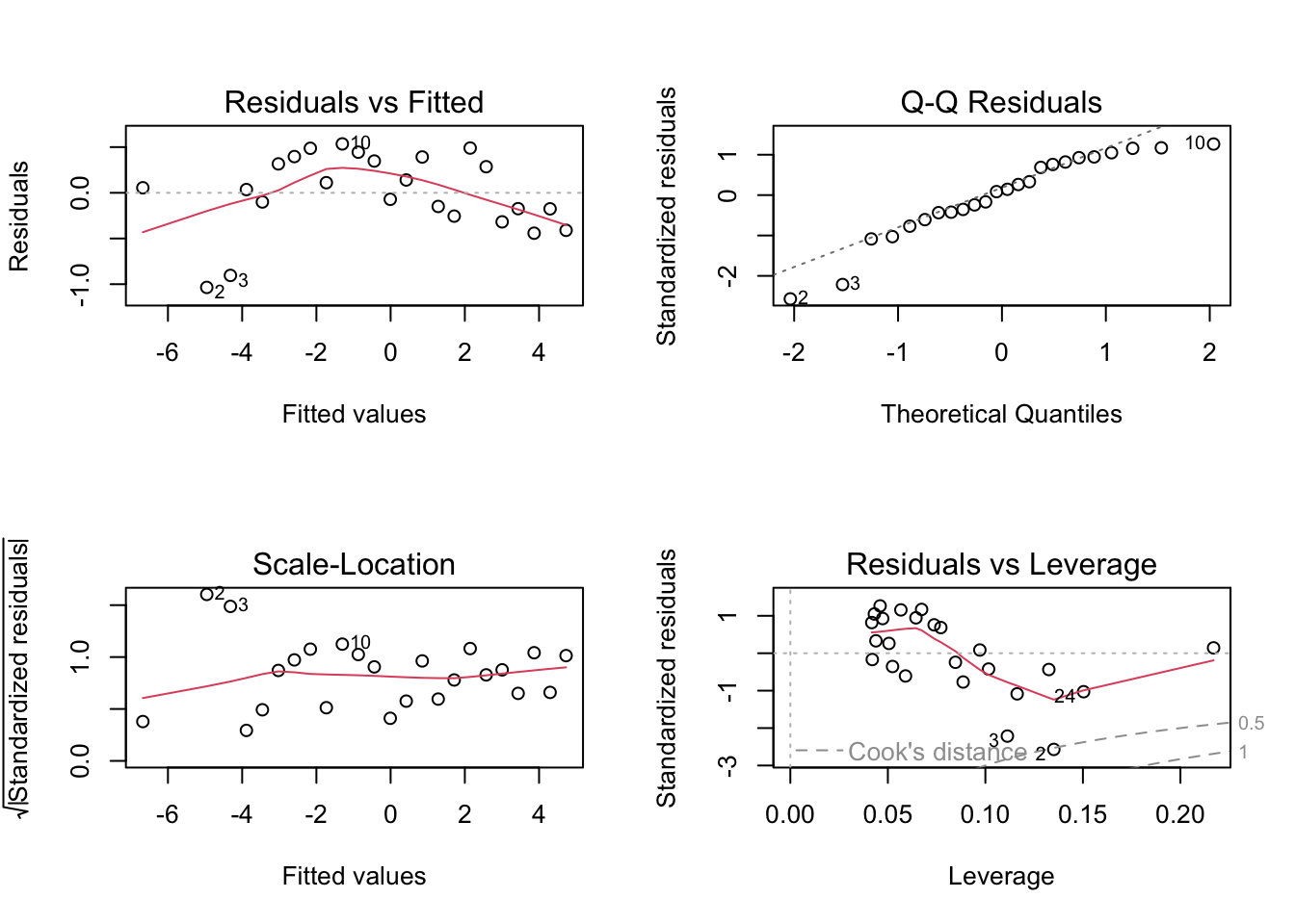
The q-q plot shows that the residuals do not seem to clearly fit a normal distribution. A popular test of normality is the Shapiro-Wilk’s test. The null hypothesis is normality.
    Shapiro-Wilk normality test

data:  residuals(m.men.1)
W = 0.92326, p-value = 0.06896
Both diagnostic tools suggest that the assumption of normality of the residuals might be questionable, however the resulting line might still be good enough for practical purposes.
8.5 Exercises
For the
ox.xlsdata example, fit a smooth spline and decide whether this is a better curve to use than the Gompertz curve. One approach is to compare the residual versus fitted plots, another is to compare the variances of the two sets of residuals.The file
alloystrength.txtrecords the compressive strength of an alloy fastener used in the construction of aircraft. Ten pressure loads, in psi, were used and different numbers of fasteners tested at each load. Is it reasonable to say that the proportion of fasteners failing is directly linearly related to the pressure load? If not, what is a more suitable transformation/model? Derive a 95% confidence interval for the proportion expected to fail at a pressure of 4000psi. At what pressure is there a 50% chance of failure?The file
Dilution.txtshows the optical density of four solutions at a sequence of dilution values. For any one of the four dilutions plot the optical against dilution, then against log10(dilution). Fit a logistic curve to the optical density values as a response to log10 dilutions and obtain 95% confidence intervals for all 4 parameter values. What are the upper and lower asymptotes? Derive a 95% confidence interval for the mean optical density at the point of inflexion of this curve. Does this curve describe the data satisfactorily and if so how would you quantify how well this logistic model describes the data?