Chapter 10 Generalised linear models
10.1 Introduction
So far we have assumed that our response data are at least approximately normally distributed, though we sometimes have had to transform to achieve this. Another common feature of our approach so far has been to seek a linear relationship between the response \(Y\) and the \(X\) variables, again perhaps after a transformation.
The theory of generalised linear models (GLMs) enables us to expand the range of distributions for the dependent response (\(Y\)) and to incorporate, as standard, a wide range of transformations linking the \(Y\) variable to the \(X\) variables. Although the underlying theory is now more complex, it provides a single unifying algorithm by which all the coefficients in our regression models can be estimated and all inferences can be made. GLMs can be thought of as introducing more flexibility to the multiple regression model we have used so far.
The first distinctive feature of GLMs is the distribution of the response variable \(Y\). GLMs allow for a normal distribution (as in ordinary multiple regression), but also for other distributions like the binomial and Poisson distributions for binary and count response variables respectively. Each of these is referred to as distribution family.
The second feature is a function (or transformation) of the mean value of \(Y\) which links it to a linear combination of the \(X\) variables. Let \(\mu\) denote the mean of \(Y\) and \(g\) denote the link function. We then have
\[g(\mu) = b_0 + b_1X_1 + b_2X_2 + \ldots + b_pX_p\] This is similar, but not identical, to regression models we have already seen after a transformation of the \(Y\) variable. The following default pairings of distribution family and link function are both theoretically convenient and practically useful.
The third distinguishing feature, which is a consequence of the first two extensions to the basic linear regression model, is that the variance of \(Y\) becomes a known function of the mean of \(Y\), \(\mu\). Denoting this function of \(\mu\) by \(V\), we have
\[Variance(Y) = \sigma^2V(\mu),\] where \(\sigma^2\) is called the dispersion parameter. It is a constant or scaling factor. For the Poisson and binomial distributions it is 1. For the normal it must be estimated from the data. In practice, for GLMs, we must specify the distribution family and the link function. After that the software package generates the same type of estimates, p-values and diagnostic plots that ordinary regression models generate. However, the underlying methodology is different and the statistical tests are different.
10.2 Deviance
With GLMs the deviance has the same pivotal role in hypothesis testing as residual sums of squares (RSS) have in ordinary regression. The deviance measures the discrepancy between the current model and the saturated model, i.e. the model which fits the data perfectly (the RSS does exactly the same). The deviance is based on so-called likelihood functions, whereas the RSS is based on fitted values. The smaller the deviance the better the current model fits the data. For GLMs with normal error and identity link the deviance is identical to the RSS. All other GLMs have their own formula for the deviance. One consequence of these formulae for the binomial and Poisson families is that the mean deviance, i.e. deviance/df(deviance), should be approximately equal to 1.
10.3 Simple linear regression as a GLM
We return to the Diffpor data used to illustrate simple linear regression. Now we analyse these data as a GLM. Note that Gaussian is a synonym for normal and the default link function is identity.
diffpor <- read.table("diffpor.txt",header=TRUE)
m.reg.1 <- lm(Diffusivity~Porosity, data=diffpor)
m.glm.1 <- glm(Diffusivity~Porosity, family=gaussian(link=identity), data=diffpor)
Note that summary(m.glm.1) and plot(m.glm.1) generate almost identical output to summary(m.reg.1) and plot(m.reg.1) used before. However, they present information about \(\sigma^2\) differently (look for “Dispersion parameter for Gaussian family …” in the first and “Residual standard error …” in the second).
Call:
glm(formula = Diffusivity ~ Porosity, family = gaussian(link = identity),
    data = diffpor)

Coefficients:
            Estimate Std. Error t value Pr(>|t|)
(Intercept)  -36.150      7.059  -5.121 5.33e-06 ***
Porosity     191.869     19.024  10.086 1.92e-13 ***
---
Signif. codes:  0 '***' 0.001 '**' 0.01 '*' 0.05 '.' 0.1 ' ' 1

(Dispersion parameter for gaussian family taken to be 72.20871)

    Null deviance: 10811  on 49  degrees of freedom
Residual deviance:  3466  on 48  degrees of freedom
AIC: 359.83

Number of Fisher Scoring iterations: 2
Call:
lm(formula = Diffusivity ~ Porosity, data = diffpor)

Residuals:
     Min       1Q   Median       3Q      Max
-22.8377  -3.6523  -0.2586   6.4514  15.0830

Coefficients:
            Estimate Std. Error t value Pr(>|t|)
(Intercept)  -36.150      7.059  -5.121 5.33e-06 ***
Porosity     191.869     19.024  10.086 1.92e-13 ***
---
Signif. codes:  0 '***' 0.001 '**' 0.01 '*' 0.05 '.' 0.1 ' ' 1

Residual standard error: 8.498 on 48 degrees of freedom
Multiple R-squared:  0.6794,    Adjusted R-squared:  0.6727
F-statistic: 101.7 on 1 and 48 DF,  p-value: 1.915e-13
The function glm provides estimates of the regression coefficients and the dispersion parameter. Although summary provides inferences based on \(t\)-tests derived from asymptotic theory, tests based on the model deviances are generally preferable for GLMs. Conceptually these work in exactly the same way as the tests based on RSS and are available from the anova function.
Analysis of Deviance Table

Model: gaussian, link: identity

Response: Diffusivity

Terms added sequentially (first to last)

         Df Deviance Resid. Df Resid. Dev      F    Pr(>F)
NULL                        49      10811
Porosity  1     7345        48       3466 101.72 1.915e-13 ***
---
Signif. codes: 0 '***' 0.001 '**' 0.01 '*' 0.05 '.' 0.1 ' ' 1Analysis of Variance Table
Response: Diffusivity
Df Sum Sq Mean Sq F value Pr(>F)
Porosity 1 7345 7345.0 101.72 1.915e-13 ***
Residuals 48 3466 72.2
---
Signif. codes: 0 '***' 0.001 '**' 0.01 '*' 0.05 '.' 0.1 ' ' 1‘NULL’ here refers to a model based only on an overall mean: \(Mean(Diff) = b_0\), its residual deviance is 10811.
‘Porosity’ here refers to the model: \(Mean(Diff) = b_0 + b_1Porosity\) and its residual deviance is 3466.
‘NULL’ is a sub-model of the ‘Porosity’ model. We can think of the ‘Porosity’ model as \(H_A\) and the ‘NULL’ model as \(H_0\) in hypothesis testing. In a previous section we said “… large values of \(RSS(sub) - RSS(full)\) suggest \(H_A\) is true. Small values suggest \(H_0\) is true.”
For GLMs we say: “large values of \(Deviance(sub) - Deviance(full)\) suggest \(H_A\) is true. Small values suggest \(H_0\) is true”. This difference in deviances is referred to in this example as the deviance due to Porosity.
Only because we are using the Gaussian family with an identity link function, i.e the same model we used previous (\(Y = a + bX + \epsilon\)), the residual deviance results here are identical to the residual sums of squares from the ordinary regression analysis.
Note that it is not always correct to say that the smaller the residual deviance the better the model describes the data. Assumptions regarding distribution and variances still have to be assessed.
10.4 Binomial GLM (logistic) regression
Returning to the menarche data set we used before, for each age group we have the total number of girls and the number among them who have had their first period.
'data.frame':   25 obs. of  3 variables:
 $ Age     : num  9.21 10.21 10.58 10.83 11.08 ...
 $ Total   : num  376 200 93 120 90 88 105 111 100 93 ...
 $ Menarche: num  0 0 0 2 2 5 10 17 16 29 ...
We want to model \(p\), the probability a girl having her first period, as a function of a single \(X\) variable, Age. The model would be
\[Y\sim Bin(N,p)\] \[\mbox{logit}(p)=b_0+b_1Age\] The response is Menarche which has a binomial distribution with parameters \(N\) and \(p\). The \(N\), the column Total, varies with each value of Age. It is worth noting that although the response is Menarche, we are modelling \(p\), the expected (mean) value of \(Y\) as linear function of the explanatory variables.
We need to create appropriate structures for the function glm when the data are binomial.
yes <- menarche$Menarche
no <- with(menarche,Total-Menarche)
y <- cbind(yes, no) #create a single 2-column object as the response
m.men2.glm <- glm(y ~ Age, family=binomial(link="logit"), data=menarche)
summary(m.men2.glm)
Call:
glm(formula = y ~ Age, family = binomial(link = "logit"), data = menarche)

Coefficients:
             Estimate Std. Error z value Pr(>|z|)
(Intercept) -21.22639    0.77068  -27.54   <2e-16 ***
Age           1.63197    0.05895   27.68   <2e-16 ***
---
Signif. codes:  0 '***' 0.001 '**' 0.01 '*' 0.05 '.' 0.1 ' ' 1

(Dispersion parameter for binomial family taken to be 1)

    Null deviance: 3693.884  on 24  degrees of freedom
Residual deviance:   26.703  on 23  degrees of freedom
AIC: 114.76

Number of Fisher Scoring iterations: 4Waiting for profiling to be done... 2.5 % 97.5 %
(Intercept) -22.786603 -19.763832
Age 1.520103 1.751327The coefficient for Age is clearly significant. However for GLMs this \(t\)-test, derived from asymptotic theory as said before, is sometimes unreliable. A better statistical test, based on changes in the deviance, is given in the anova summary. However, for binomial and Poisson data, where the dispersion parameter must be 1, we have to use Chi-squared (\(\chi^2\)) tests.
Analysis of Deviance Table

Model: binomial, link: logit

Response: y

Terms added sequentially (first to last)

     Df Deviance Resid. Df Resid. Dev  Pr(>Chi)
NULL                    24     3693.9
Age   1   3667.2        23       26.7 < 2.2e-16 ***
---
Signif. codes:  0 '***' 0.001 '**' 0.01 '*' 0.05 '.' 0.1 ' ' 1
The test statistic, Deviance, has a \(\chi^2\) distribution. Chi-squared distributions have a single parameter, degrees of freedom. Large values of this test statistic provide evidence away from the null hypothesis that (in our case) \(b_1=0\). In the output we can see that the \(p\)-value given by Pr(\(\chi^2 > 3667.2\)) is \(\approx 0\) (\(3667.2 = 3693.9-26.7\)). Hence the result is highly significant and we should keep Age in the model.
Before looking at the diagnostic plots we note that the mean residual deviance, the scaled deviance, is \(26.7/23 = 1.16\). Binomial and Poisson models both have true dispersion (mean deviance) values of 1, thus the fact that the estimate from the model is close to 1 is a good sign.
# Copy of current graphic parameters
oldpar <- par()
# Modify them to do a 2x2 matrix of graphs
par(oma = c(0, 0, 0, 0), mfrow=c(2, 2))
plot(m.men2.glm)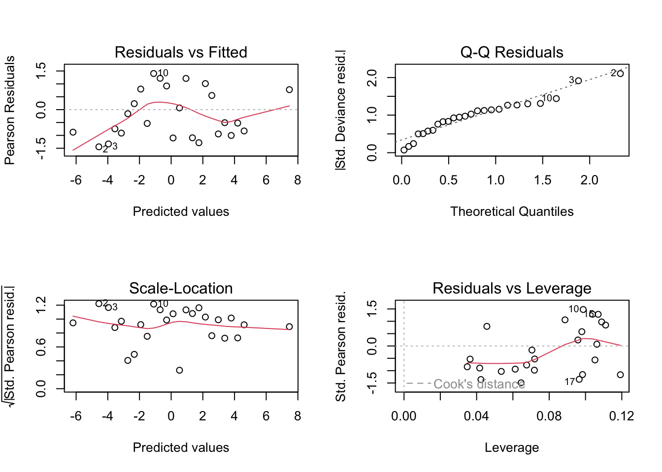
These plots show slightly improved residual behaviour over fitting an ordinary linear regression model to the logit transformed data as we did before. Another advantage of GLMs is that the fitted values are given in the natural scale for the response variable. So in this case in terms of \(p\), as opposed to the transformed scale logit(\(p\)).
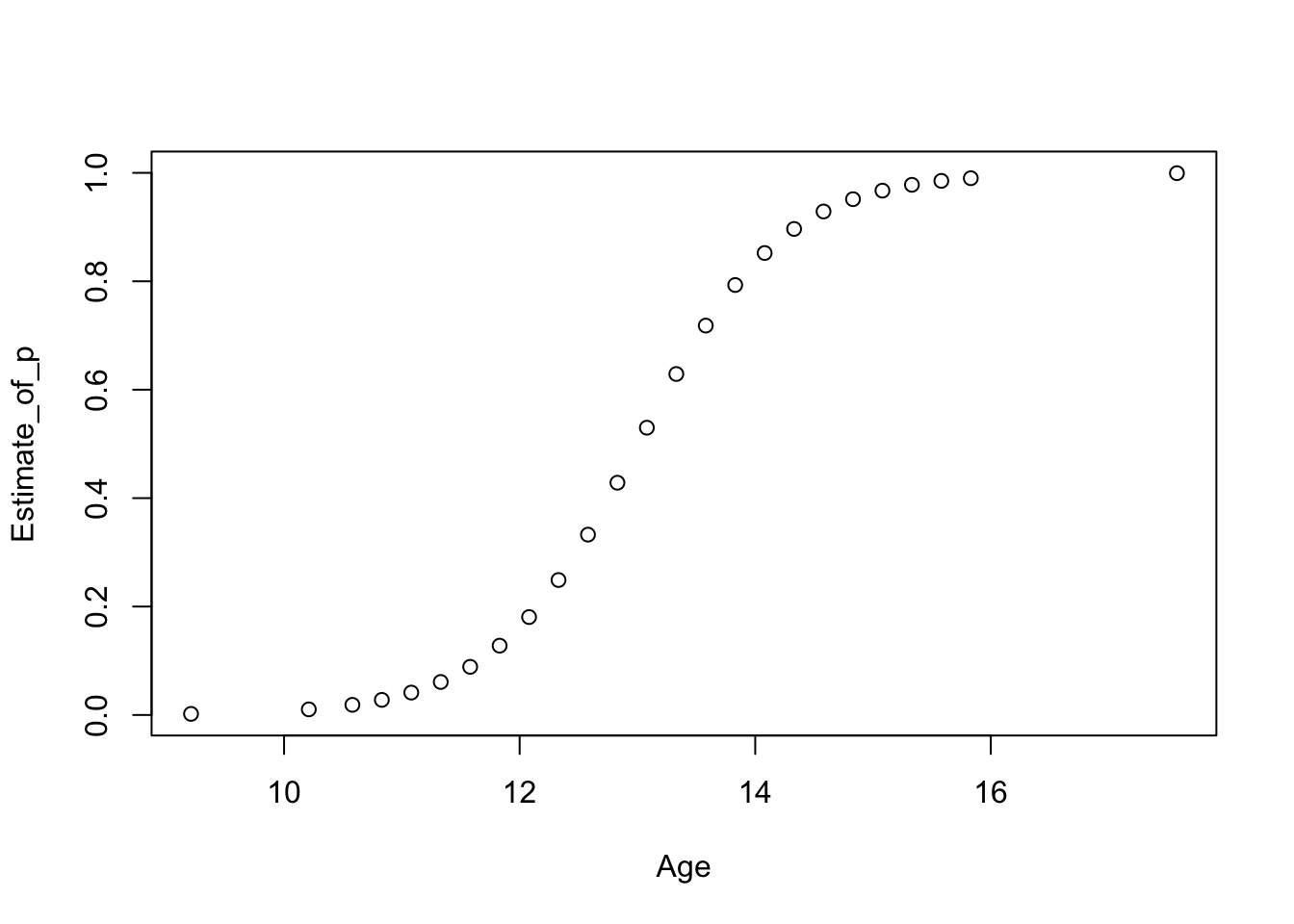
Predictions (probabilities \(p\) in this case) for ages from 10 to 16 are easily obtained using predict as usually.
$fit
          1           2           3           4
0.007342463 0.162087859 0.834955317 0.992498323

$se.fit
          1           2           3           4
0.001380336 0.011886625 0.011739359 0.001386084

$residual.scale
[1] 1
10.5 Poisson GLM regression
The cans data set refers to the number of cans sold in a vending machine each week, along with the average temperature for that week.
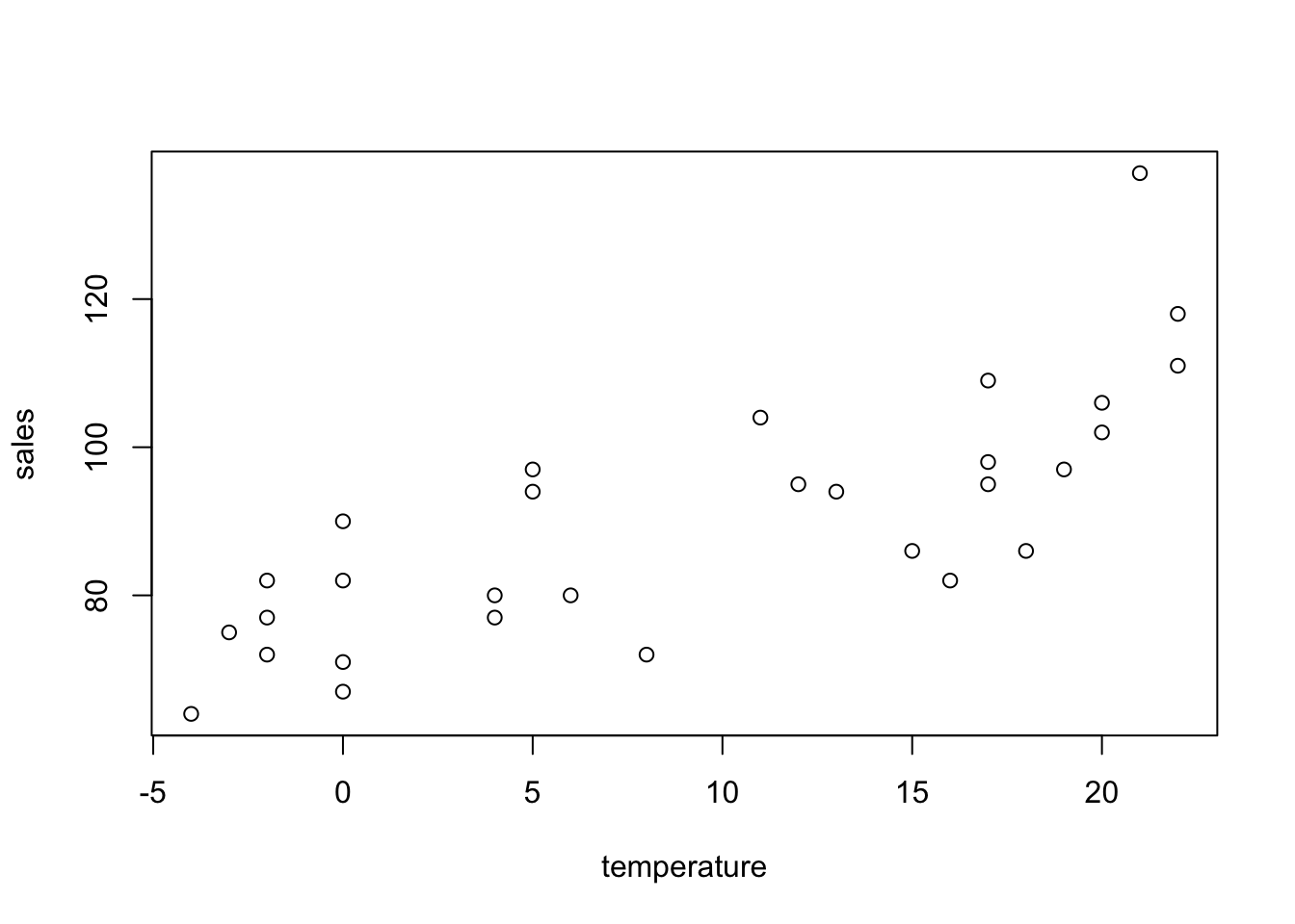
The sales data are counts and they are likely to follow a Poisson distribution. We want to see if mean weekly sales can be modelled as a function of temperature. The default link function for Poisson data is the natural logarithm (\(\ln\)).
Letting \(Y\) denote the number of cans sold in a week, we model \(Y\) as a Poisson variable with mean \(\lambda\) as
\[Y\sim Poisson(\lambda)\] \[\ln\lambda=b_0+b_1temperate\]
Call:
glm(formula = sales ~ temperature, family = poisson, data = cans)
Coefficients:
Estimate Std. Error z value Pr(>|z|)
(Intercept) 4.340983 0.030253 143.489 < 2e-16 ***
temperature 0.016024 0.002219 7.222 5.14e-13 ***
---
Signif. codes: 0 '***' 0.001 '**' 0.01 '*' 0.05 '.' 0.1 ' ' 1
(Dispersion parameter for poisson family taken to be 1)
Null deviance: 84.661 on 29 degrees of freedom
Residual deviance: 32.047 on 28 degrees of freedom
AIC: 225.77
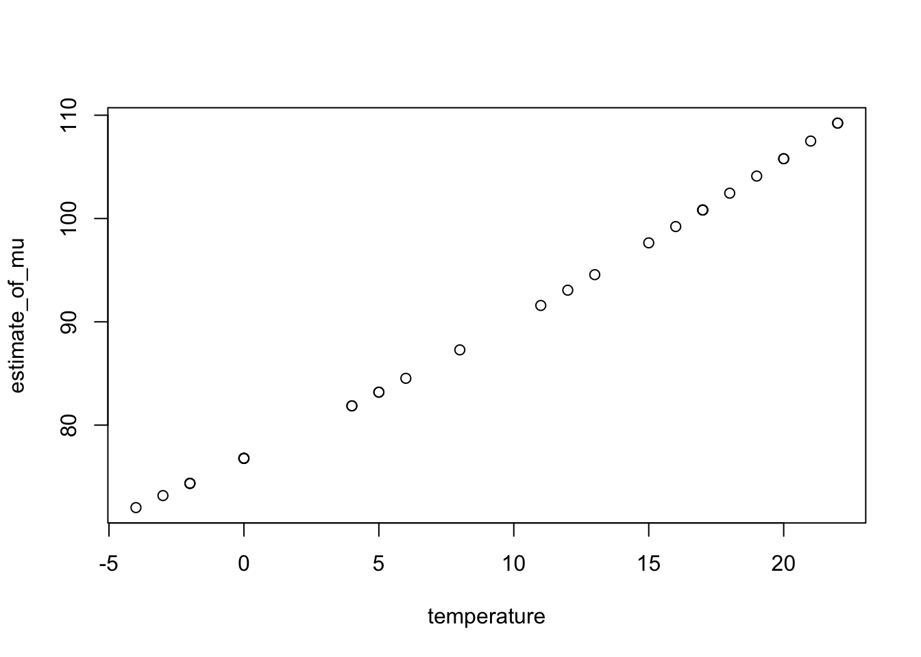
Number of Fisher Scoring iterations: 4The fitted model involves a Poisson distribution for weekly sales with parameter \(\lambda\) where \(\ln\lambda = 4.34 - 0.0160temperature\). The \(t\)-test suggests temperature is strongly significant but again it is better to use the \(\chi^2\) test.
Analysis of Deviance Table

Model: poisson, link: log

Response: sales

Terms added sequentially (first to last)

            Df Deviance Resid. Df Resid. Dev  Pr(>Chi)
NULL                           29     84.661
temperature  1   52.614        28     32.047 4.059e-13 ***
---
Signif. codes:  0 '***' 0.001 '**' 0.01 '*' 0.05 '.' 0.1 ' ' 1
Note that the dispersion (mean residual deviance) is estimated as \(32.05/28\), approximately 1, the true value we would expect when the data follow a Poisson distribution. The resulting \(p\)-value is very small and hence suggests that temperature is associated with sales. The diagnostic plots indicate a reasonable fit.
# Copy of current graphic parameters
oldpar <- par()
# Modify them to do a 2x2 matrix of graphs
par(oma = c(0, 0, 0, 0), mfrow=c(2, 2))
plot(m.can.glm)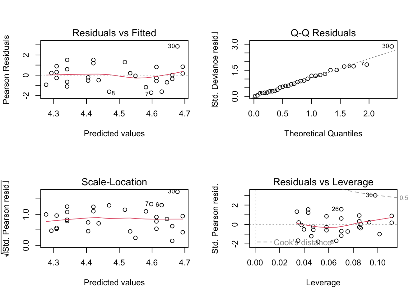
We can obtain estimated mean sales with temperature.
10.6 Explanatory factor variables, offsets and interaction effects
We extend GLMs to include categorical variables, which must be introduced as factors into the glm function. We also include an offset, that is a variable in the linear predictor whose coefficient we insist takes the value 1. An offset is used to account for a baseline value for the response variable to make the values of this latter comparable between individuals.
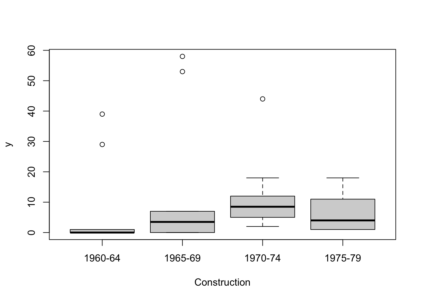
The data file Damage.txt contains the number of times waves caused damage to forward sections of cargo-carrying ships. To set standards of hull construction, the damage risk associated with various factors is assessed.
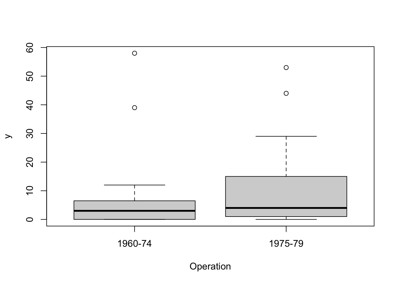
The following plots show wave damage in cargo ships by ship type, construction date, and time of occurrence.
ships <- read.table("ships.txt",header=TRUE, stringsAsFactors = TRUE)
plot(ships$Type, ships$Damage, xlab= "Type",)
Damage measures are counts and we begin by assuming they have a Poisson distribution. We want to know if the mean number of damage incidents is affected by Type, Construct or Operation, or some combination of these. Our first model is
\[\log(\lambda) = mean + Effect(Type) + Effect(Construct) + Effect(Operation)\] However we also have data on how long each ship was in service, in months, and it would seem more sensible to model the mean number of incidents per month, i.e. to model \(\log(\lambda/Service)\). But \(\log(\lambda/Service) = \log\lambda-\log(Service)\). So the model becomes
\[\log(\lambda) = mean + log(Service) +Effect(Type) + Effect(Construct) + Effect(Operation)\] We now have \(\log(Service)\) in the model as an offset (its coefficient is fixed at 1).
ships$logS  <- log(ships$Service)
m.ship.glm <-
  glm(Damage ~ offset(logS) + Type + Construct + Operation,
      family = poisson,
      data = ships)
anova(m.ship.glm, test="Chisq")
Analysis of Deviance Table
Model: poisson, link: log
Response: Damage
Terms added sequentially (first to last)
Df Deviance Resid. Df Resid. Dev Pr(>Chi)
NULL 33 146.328
Type 4 55.439 29 90.889 2.629e-11 ***
Construct 3 41.534 26 49.355 5.038e-09 ***
Operation 1 10.660 25 38.695 0.001095 **
---
Signif. codes: 0 '***' 0.001 '**' 0.01 '*' 0.05 '.' 0.1 ' ' 1We see that all three factors, Type, Construction and Operation affect Damage. It can happen that the effects of a factor vary according to the levels of another factor (or more generally according to the values of another covariate). This is called an interaction effect and we can include this in the model, for example there is some evidence in the area about a Type by Construction interaction (this is a 2-way interaction). Single 2-way interactions are specified with the : operator in R formulae.
m.ship.glm.int <-
  glm(
    Damage ~ offset(logS) + Type + Construct + Operation + Type:Construct,
    family = poisson,
    data = ships
  )
anova(m.ship.glm.int, test="Chisq")
Analysis of Deviance Table
Model: poisson, link: log
Response: Damage
Terms added sequentially (first to last)
Df Deviance Resid. Df Resid. Dev Pr(>Chi)
NULL 33 146.328
Type 4 55.439 29 90.889 2.629e-11 ***
Construct 3 41.534 26 49.355 5.038e-09 ***
Operation 1 10.660 25 38.695 0.001095 **
Type:Construct 12 24.108 13 14.587 0.019663 *
---
Signif. codes: 0 '***' 0.001 '**' 0.01 '*' 0.05 '.' 0.1 ' ' 1A full model considering all main effects and possible interactions (2-way and 3-way in this case) is specified as follows.
m.ship.glm.int2 <-
  glm(
    Damage ~ offset(logS) + Type*Construct*Operation,
    family = poisson,
    data = ships
  )
anova(m.ship.glm.int2, test="Chisq")
Analysis of Deviance Table
Model: poisson, link: log
Response: Damage
Terms added sequentially (first to last)
Df Deviance Resid. Df Resid. Dev Pr(>Chi)
NULL 33 146.328
Type 4 55.439 29 90.889 2.629e-11 ***
Construct 3 41.534 26 49.355 5.038e-09 ***
Operation 1 10.660 25 38.695 0.001095 **
Type:Construct 12 24.108 13 14.587 0.019663 *
Type:Operation 4 6.066 9 8.521 0.194267
Construct:Operation 2 1.664 7 6.856 0.435103
Type:Construct:Operation 7 6.856 0 0.000 0.443978
---
Signif. codes: 0 '***' 0.001 '**' 0.01 '*' 0.05 '.' 0.1 ' ' 1Along with the main effects of the factors, following the usual statistical significance criteria, the only significant interaction is that between Type by Construction. So the model could be simplified to m.ship.glm.int above.
In fact, the following exploratory plots of the data (produced using the package ggplot2) would have already suggested this potential interaction effect, the effect of Type on Damage appears to change depending on Construct.
library(ggplot2)
ggplot(aes(x=Type, y=Damage, fill = Type), data = ships) +
  facet_wrap(~Construct) +
  geom_boxplot() +
  theme_bw()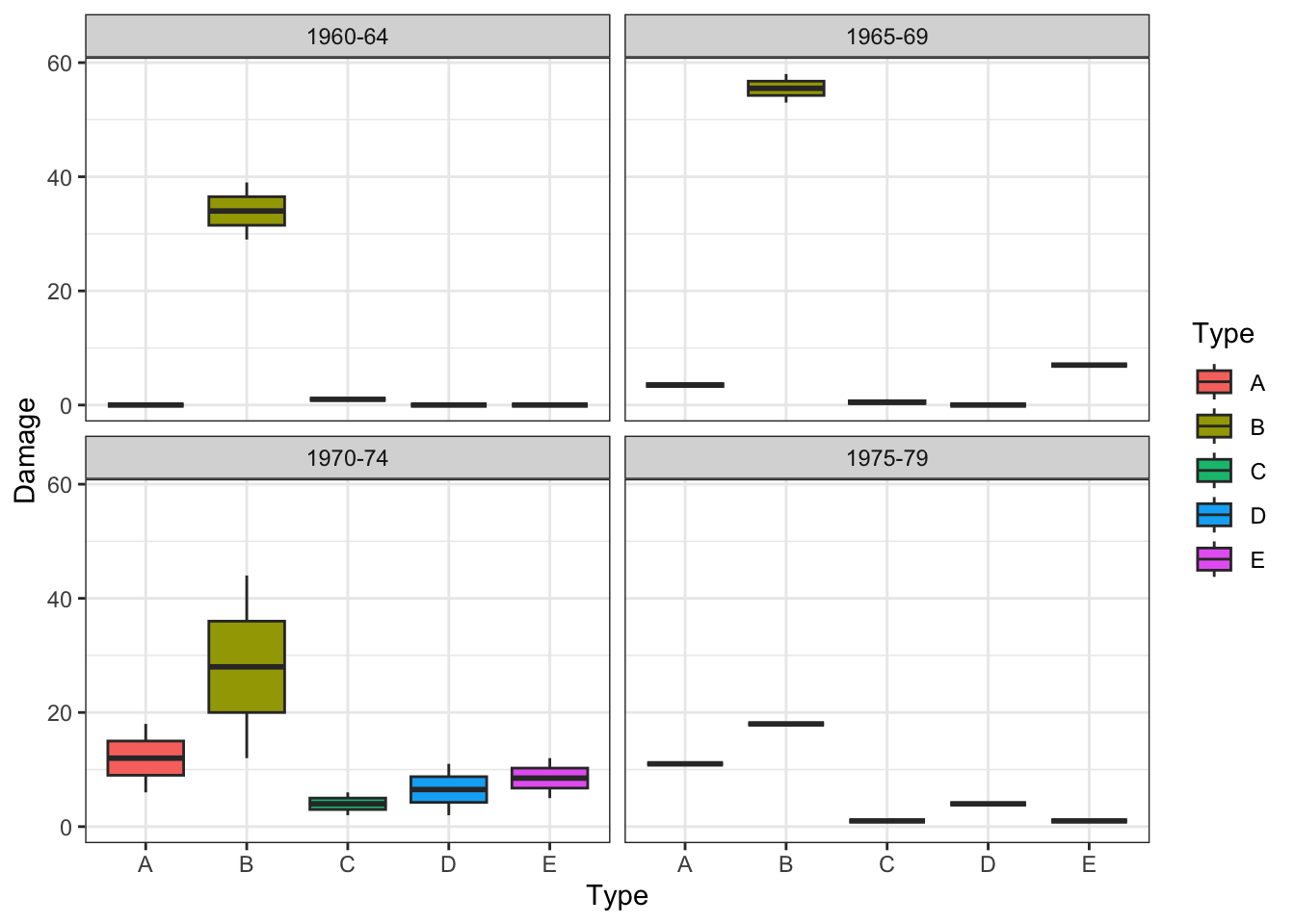
We have illustrated the inclusion of interactions here, but this applies to any regression and ANOVA model. However, note that including too many interactions can lead to fitting problems and complicates the interpretation of the models. So their specification should be better guided by sensible considerations in the context of application.
Finally note that we have illustrated the use of GLMs with gaussian, binomial and Poisson data distributions, but other families can be similarly specified though the family argument of the glm function (see ?family).
10.7 Exercises
The data file
pigs.txtcontains the number of occurrences of various types of behaviour among pigs in pens. Not all pens had the same number of pigs and only totals were recorded as it was not possible to observe each pig individually. The pens either had straw or did not have straw. Prior to the experiment the pigs had been housed in three different mixing treatments which related to what extent the animals remained with their siblings and the size of group they were living in. Using a Poisson distribution to model the counts, with an offset for the number of pigs in the pen, and a log link, decide whether straw or mixing or an interaction between straw and mixing affected (a) the feeding counts (b) the drinking counts (c) the ‘up’ counts. Check that your final models have well behaved residuals.In the file
drop.txtthere are data about 36 batches of 8 potato tubers. These were dropped from various heights onto bars to test their resistance to splitting. How do tuber weight and drop height affect the probability of a tuber splitting?