Chapter 7 Linear regression

7.1 Introduction

In brief regression analysis is the study of the relationships between variables, typically one (or several) playing the role of response (dependent) variable and one or several playing the role of explanatory (independent) variables or predictors. We may want to do this for a number of reasons:

We are interested in understanding the association between variables.
We want to know how best to predict the value of a variable given the values of others, and how good this prediction is.
We may want to investigate whether any relationship exists.

We are careful not to use words that imply that one variable causes changes in another. It may be so, but an association does not prove causation. Such things can only be established by careful interpretation of appropriately designed experiments, if this is possible.

Let us refer to the explanatory variable as \(X\) and the response variable as \(Y\). We assume that \(X\) is known exactly. Some adjustment would need to be made to our results if it was believed to be subject to measurement error. We suppose that values of \(Y\) are random with a mean which is some function of \(X\):

\[Y=f(X)+\epsilon\]

where \(\epsilon\) is a random variable independent of \(X\) and usually assumed to have a \(N(0,\sigma^2)\) distribution. For linear regression, we assume that \(f(X)\) is a linear function, and so

\[Y=a + bX + \epsilon\]

Here the parameter \(a\) is the intercept: the mean value of \(Y\) when \(X\) is zero. The parameter \(b\) is the slope of the relationship: the average amount by which \(Y\) changes when \(X\) increases by 1.

We don’t know the true values of \(a\) and \(b\), but regression enables us to find the values of \(a\) and \(b\) which best fit the data. The least squares solution finds the values of \(a\) and \(b\) which minimise the sum of squared residuals. The following figure summarises the basic elements of simple linear regression.

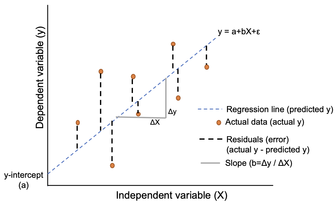
(https://www.reneshbedre.com/blog/linear-regression.html)

We illustrate these ideas by looking at some data on simulated soil diffusivity (diffpor.txt). The observations consist of 50 values of porosity and diffusivity and are plotted below.

We show below the output produced by R.

diffpor <- read.table("diffpor.txt", header = TRUE)
# use plotting character 20 (filled circle), expanded by factor 2
plot(diffpor$Porosity,
     diffpor$Diffusivity,
     cex = 2,
     pch = 20)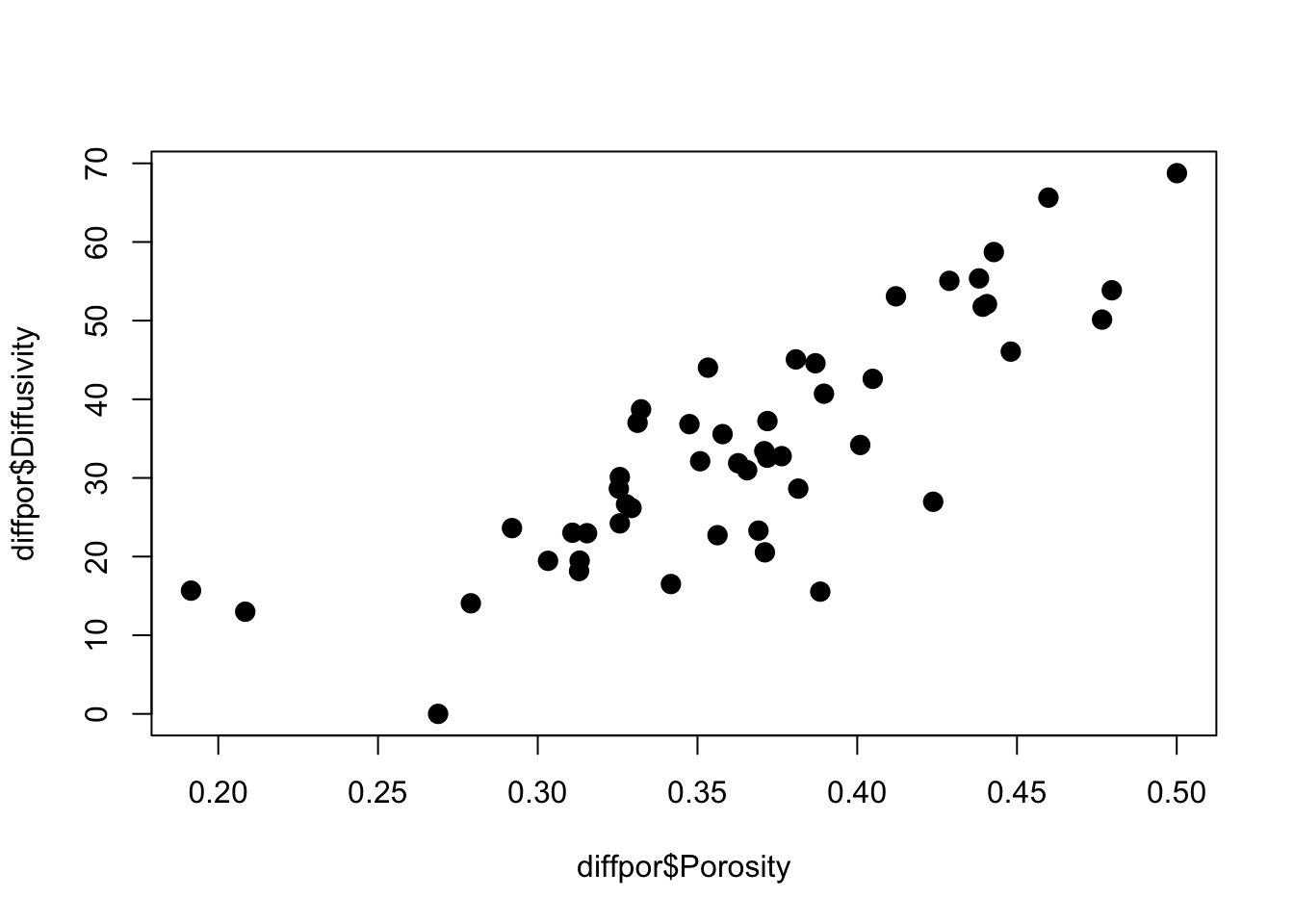

m.reg.1 <- lm(Diffusivity ~ Porosity, data = diffpor)
summary(m.reg.1)


Call:
lm(formula = Diffusivity ~ Porosity, data = diffpor)

Residuals:
     Min       1Q   Median       3Q      Max 
-22.8377  -3.6523  -0.2586   6.4514  15.0830 

Coefficients:
            Estimate Std. Error t value Pr(>|t|)    
(Intercept)  -36.150      7.059  -5.121 5.33e-06 ***
Porosity     191.869     19.024  10.086 1.92e-13 ***
---
Signif. codes:  0 '***' 0.001 '**' 0.01 '*' 0.05 '.' 0.1 ' ' 1

Residual standard error: 8.498 on 48 degrees of freedom
Multiple R-squared:  0.6794,    Adjusted R-squared:  0.6727 
F-statistic: 101.7 on 1 and 48 DF,  p-value: 1.915e-13

There are several parts to the output:

A description of the model being fitted.
A summary of the distribution of the residuals.
The regression coefficients and their standard errors. The coefficients are the values of \(a\) and \(b\) in the regression equation. The standard errors indicate how much they are subject to sampling variability (in other words they indicate the precision with which \(a\) and \(b\) have been estimated). The \(t\)-statistics are the ratios of the coefficient to their standard errors, and provide a way of assessing whether the coefficients differ significantly from zero. P-values are also given. Note that if the parameter \(b = 0\), this implies no relationship between \(X\) and \(Y\). If \(a = 0\), then \(Y\) is directly proportional to \(X\), and the line passes through the origin.
Some summaries of goodness-of-fit. These indicate how well the regression model describes the data. In other words, how much of the variation in \(Y\) can be accounted for by variation in \(X\), and how much remains.
- Multiple \(R^2 = 1 - (\mbox{residual sum of squares}) / (\mbox{total sum of squares})\)
- Adjusted \(R^2 = 1 - (\mbox{residual mean square}) / (\mbox{total mean square})\)
both \(R^2\) are expressed as a value in \([0, 1]\). The adjustment referred to has the effect of offsetting the tendency for \(R^2\) to increase with additional explanatory variables in multiple regression (i.e. more than one \(X\) variable), even when they have no explanatory power. To obtain the sums of squares and mean squares we need to use the aov function (see below).
Residual Standard Error is the estimate of \(\sigma\), the standard deviation of the residuals. The \(\sigma\) quantifies how spread out around the regression line the data values are.
\(F\)-Statistic refers to a test of whether the fitted model is a significant improvement over the mean of \(Y\) in predicting the individual \(Y\) values. In the case of simple linear regression the significance of the \(F\)-statistic is identical to the significance of \(t\)-test for \(b = 0\).

In addition to using lm to obtain estimates of the regression line parameters, we can use confint to compute confidence intervals for the parameters.

confint(m.reg.1, level = .95)

                2.5 %   97.5 %
(Intercept) -50.34275 -21.9564
Porosity    153.61845 230.1197

7.2 Partitioning the data variation

summary(aov(m.reg.1))

            Df Sum Sq Mean Sq F value   Pr(>F)    
Porosity     1   7345    7345   101.7 1.92e-13 ***
Residuals   48   3466      72                     
---
Signif. codes:  0 '***' 0.001 '**' 0.01 '*' 0.05 '.' 0.1 ' ' 1

The aov (analysis of variance) function partitions the total variation in the \(Y\) values, \(\sum_{i=1}^n(Y_i-\bar{Y})^2\), into two components: the regression sum of squares (SS), \(\sum_{i=1}^n(\hat{Y}_i-\bar{Y})^2\), and the residual sum of squares, \(\sum_{i=1}^n(Y_i-\hat{Y}_i)^2\). In a good model, one that describes the data well, the regression sum of squares will be relatively large and the residual sum of squares will be relatively small.

\[\sum_{i=1}^n(Y_i-\bar{Y})^2 = \sum_{i=1}^n(\hat{Y}_i-\bar{Y})^2 + \sum_{i=1}^n(Y_i-\hat{Y}_i)^2\] Associated with each sum of squares is the degrees of freedom, generally 1 fewer than the number of terms contributing to the sum of squares.

For the Total SS, there are \(n\) values, so df(total) \(= n-1\). For the Regression SS there are two terms in the regression model, so df(reg) \(= 2-1\) or 1. The Residual df is what is left after fitting the model, namely \((n-1)-(2-1)\) or \((n-2)\).

The term mean squares (MS) refers to the sum of squares divided by its degrees of freedom. Mean squares can be thought of as variances.

Mean Squares (Total) \(= \sum_{i=1}^n(Y_i-\bar{Y})^2 / (n-1) =\) variance (\(Y\))

Mean Squares (Regression) \(= \sum_{i=1}^n(\hat{Y}_i-\bar{Y})^2 / 1 =\) variance (regression)

Mean Squares (Residual) \(= \sum_{i=1}^n(Y_i-\hat{Y}_i)^2 / (n-2) =\) variance (residuals)

The \(F\)-statistic from the lm function and the \(F\)-Ratio from the aov function are the same thing, namely

\[F=\frac{MS(regression)}{MS(Residual)}\] For a good regression model this ratio will be greater than 1.The larger this ratio, the better the model describes the data. The closer the \(F\)-ratio is to one, the less the variation about the regression line and the variation among the residuals are distinguishable.

The \(F\) can be thought of as a signal-to-noise ratio, and it is also the test statistic to test the hypotheses \(H_0: b = 0\) versus \(H_A: b\neq 0\). Large positive values of \(F\) are evidence away from \(H_0\) towards \(H_A\).

Under \(H_0\) \(F\) has an \(F\) probability distribution. Associated with the \(F\) distribution are two parameters, the numerator (regression) degrees of freedom and the denominator (residual) degrees of freedom. In our case these parameter values are 1 and \((n-2) = 48\).

Features of the \(F\) distribution can be obtained in R in the usual way by the functions rf, pf, qf and df, analogous to the functions rnorm, pnorm, qnorm and dnorm.

7.3 Diagnostic plots

We can examine a plot including the fitted line. This should give us a good idea of how well the regression describes the data, or whether there are any problems with the fit.

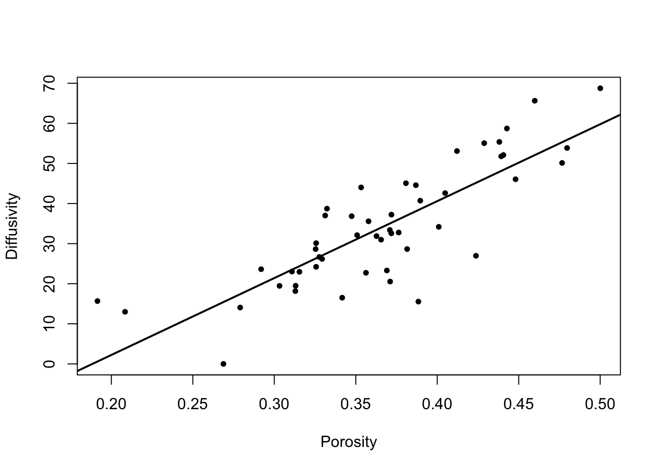
with(diffpor,plot(Porosity,Diffusivity,pch=20))
abline(m.reg.1,lwd=2) #add a line to current plot

However, diagnostic plots, based on the regression residuals, are designed to highlight the specific nature of any problems with the fitted regression model. They allow us to investigate whether each of the underlying assumptions of the regression model are justified. Specifically we assess whether the residuals have a constant variance and whether they are approximately normally distributed.

Common diagnostic plots based on residuals can be obtained by using plot on the lm object.

# Copy of current graphic parameters
oldpar <- par()
# Modify them to do a 2x2 matrix of graphs
par(oma = c(0, 0, 0, 0), mfrow=c(2, 2))
plot(m.reg.1)

# Revert to original settings
par(oldpar)

The residuals are the differences between the observations and their fitted values from the regression line. There should ideally be no pattern discernible in the residuals. If there were, it could be incorporated in the model. The best way to examine the residuals for pattern is to plot residuals against fitted values. This is shown in the top left plot. The only comment of note here seems to be that the residuals for the two lowest fitted values are positive, and by looking at the previous figure also, we may see a hint of curvature in the relationship. We might explore further by omitting these two observations and seeing how the fitted curve is affected (see below). Another pattern to look out for is residuals becoming more variable with increasing fitted value. This might indicate a need to transform \(X\) and/or \(Y\).

It is assumed in much of linear regression that the residuals have a normal distribution. This can be checked by examining a q-q plot of residuals (top right graph). The departure from a straight line here is not too bad though the systematic deviation from the straight line for the lower porosity values is worth noting. Serious departure from normality might point to a need to transform the variables, or to fit a generalized linear model (GLM).

It is straightforward to get the residuals and fitted values explicitly from a regression.

residual <- m.reg.1$residuals     #could also use resid(reg1)
fitted <- m.reg.1$fitted.values   #could also use fitted(reg1)
plot(fitted,residual)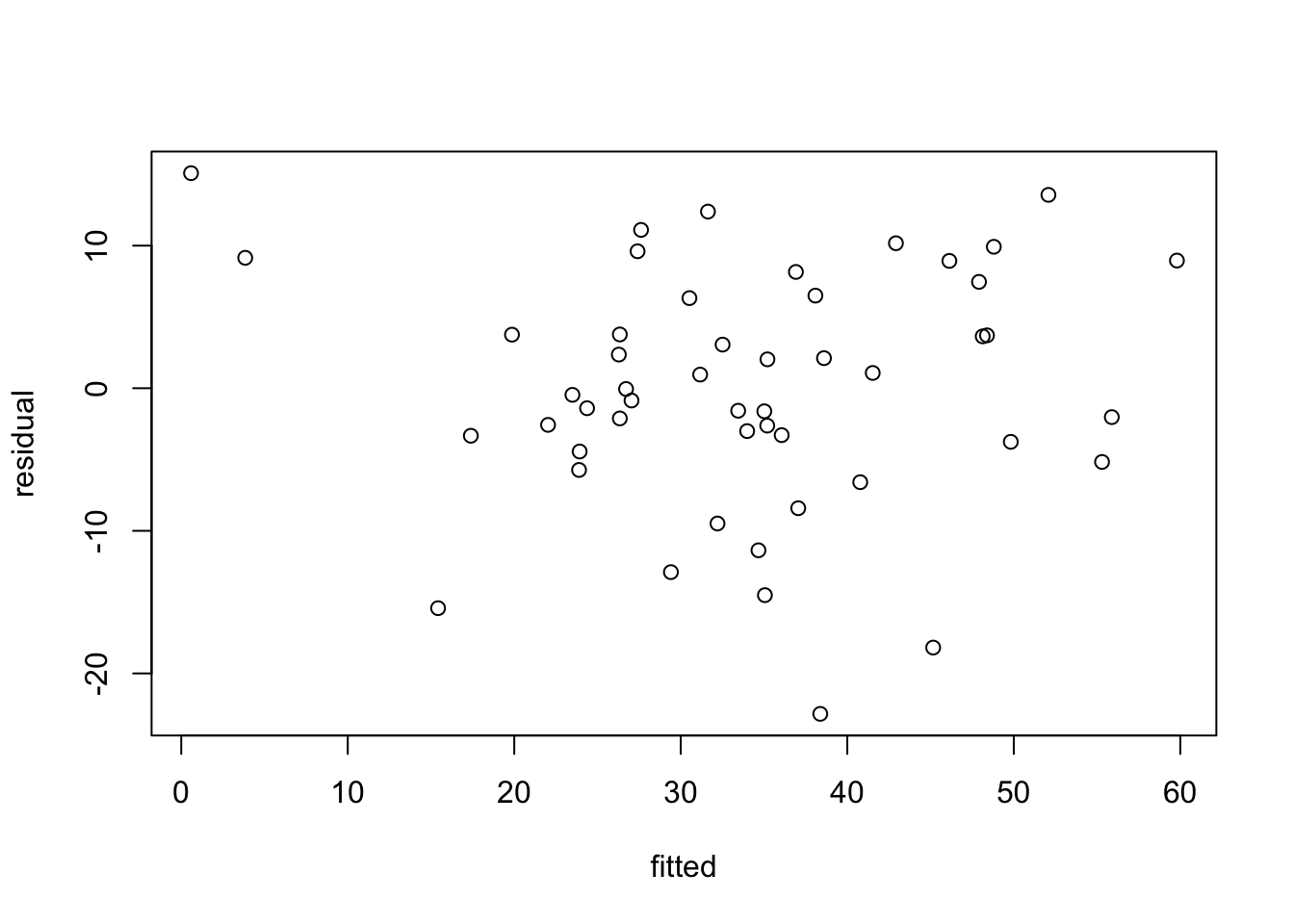

There are other measures relevant to regression diagnostics. Leverage measures how far a point is from the centre of the independent (or explanatory) variable(s), that is the \(X\) variable(s). A point with high leverage need not necessarily indicate a problem, but it is always worth checking whether it is distorting the regression line. A point whose removal from the data set causes a large change in the regression equation is said to have high influence. Cook’s \(D\) statistic is a popular measure of influence: a value greater than 1 suggests high influence.

7.4 Prediction

Sometimes the reason for deriving a regression line is to predict or estimate the value of the response variable at specific values of the independent variable. In general terms, given a new set of \(X\) values, we want to predict the corresponding \(Y\) values. These predictions are best accompanied by a confidence interval, to give an indication of the precision of our estimates.

We must distinguish between a confidence interval for the mean value of \(Y\), and the confidence interval for a single value of \(Y\), called the prediction interval in R. The estimate is the same in both cases, but the interval will be wider for the prediction of a single instance of \(Y\) rather for the mean value of \(Y\). To understand the difference between these two situations consider the use of life expectancy tables. As an individual you are interested in finding the estimate of your own life expectancy and want a confidence interval for that single value estimate. From a life assurance company’s perspective interest lies in average life expectancies and confidence intervals for estimates of these averages.

newvalues <- c(.25, .3, .35, .4, .45, .5)
newPorosity <- data.frame(Porosity = newvalues)
ci <- predict(m.reg.1, newPorosity, interval = "confidence")
pi <- predict(m.reg.1, newPorosity, interval = "prediction")

options.default <- options()    #save the default settings
options(digits = 3)     #restrict the number of digits printed
ci

   fit   lwr  upr
1 11.8  6.78 16.9
2 21.4 17.93 24.9
3 31.0 28.52 33.5
4 40.6 37.85 43.3
5 50.2 46.16 54.2
6 59.8 54.11 65.5

pi

   fit   lwr  upr
1 11.8 -6.00 29.6
2 21.4  3.97 38.8
3 31.0 13.74 48.3
4 40.6 23.29 57.9
5 50.2 32.64 67.7
6 59.8 41.78 77.8

options(options.default)    #reset to the default settings

We can use the R function matplot (matrix plot) to plot several variables simultaneously. Here we plot all the columns of ci and pi against newvalues.

# Confidence Interval for the mean value of Diffusivity
matplot(newvalues,
        ci,
        type = "l",
        col = "blue",
        lty = 2)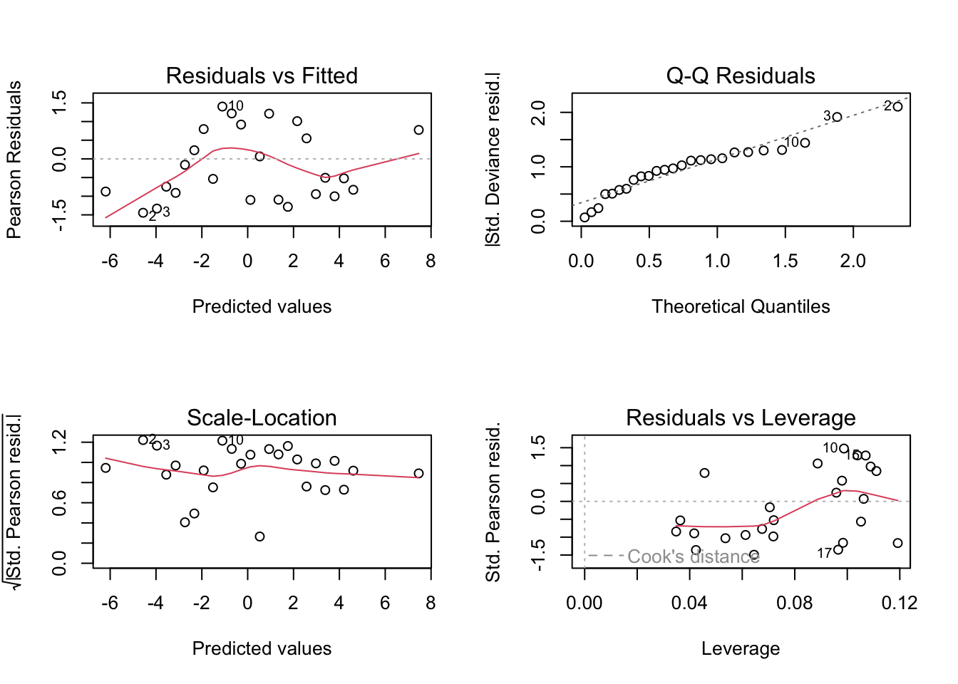

# Confidence Intervals for the mean (blue)
# and predicted (green) values of Diffusivity 
matplot(newvalues,
        ylab = "",
        ci,
        type = "l",
        col = "blue",
        lty = c(1, 2, 2))
matplot(
  newvalues,
  pi,
  type = "l",
  col = "green",
  lty = c(1, 2, 2),
  add = TRUE
)

7.5 Omitting specific data values

We mentioned above the possibility of investigating the effect of excluding the two observations with lowest porosity from the regression.

m.reg2 <- lm(Diffusivity~Porosity, subset=(Porosity>0.25), data=diffpor)
summary(m.reg2)


Call:
lm(formula = Diffusivity ~ Porosity, data = diffpor, subset = (Porosity > 
    0.25))

Residuals:
     Min       1Q   Median       3Q      Max 
-22.8058  -3.7663   0.8661   5.7562  13.4663 

Coefficients:
            Estimate Std. Error t value Pr(>|t|)    
(Intercept)  -47.744      8.086  -5.905 4.02e-07 ***
Porosity     221.637     21.477  10.320 1.48e-13 ***
---
Signif. codes:  0 '***' 0.001 '**' 0.01 '*' 0.05 '.' 0.1 ' ' 1

Residual standard error: 8.098 on 46 degrees of freedom
Multiple R-squared:  0.6984,    Adjusted R-squared:  0.6918 
F-statistic: 106.5 on 1 and 46 DF,  p-value: 1.481e-13

We see that the slope seems to be different from the estimate based on all the data, namely 192.0. However there is a large amount of uncertainty with these estimates (\(se=21\), approximately). The diagnostic plots (not shown) should play a bigger part in determining which the more appropriate model is. We note in passing that the goodness-of-fit statistics have moved in the direction of improvement: the residual standard error has decreased and adjusted \(R^2\) has increased despite the use of two data points fewer. This supports our suspicions that the relationship may not be linear over the full range of porosities.

7.6 Transformation to linearity

Some other experiments have suggested that a relationship

\[\mbox{Diffusitivity} = a + b\mbox{Porosity}^2 + \epsilon\] may be appropriate. We can fit this using linear regression, since the relationship is linear in porosity squared.

diffpor$Porosity2 <- diffpor$Porosity^2
m.reg3 <- lm(Diffusivity~Porosity2, data=diffpor)
summary(m.reg3)


Call:
lm(formula = Diffusivity ~ Porosity2, data = diffpor)

Residuals:
     Min       1Q   Median       3Q      Max 
-22.0466  -4.7285   0.5286   4.6551  13.5114 

Coefficients:
            Estimate Std. Error t value Pr(>|t|)    
(Intercept)   -3.367      3.658   -0.92    0.362    
Porosity2    271.436     25.221   10.76 2.16e-14 ***
---
Signif. codes:  0 '***' 0.001 '**' 0.01 '*' 0.05 '.' 0.1 ' ' 1

Residual standard error: 8.123 on 48 degrees of freedom
Multiple R-squared:  0.707, Adjusted R-squared:  0.7009 
F-statistic: 115.8 on 1 and 48 DF,  p-value: 2.163e-14

We see that the fit has improved (slightly higher adjusted \(R^2\) and slightly lower residual standard error).

A final point to note is that the non-significant constant is coherent with the subject matter theory, since it is expected that zero porosity requires zero diffusivity. We can force the constant to be zero in the model.

m.reg4 <- lm(Diffusivity~0+Porosity2,data=diffpor)
summary(m.reg4)


Call:
lm(formula = Diffusivity ~ 0 + Porosity2, data = diffpor)

Residuals:
     Min       1Q   Median       3Q      Max 
-22.0880  -4.7222  -0.4917   5.7099  12.9047 

Coefficients:
          Estimate Std. Error t value Pr(>|t|)    
Porosity2  249.396      7.909   31.53   <2e-16 ***
---
Signif. codes:  0 '***' 0.001 '**' 0.01 '*' 0.05 '.' 0.1 ' ' 1

Residual standard error: 8.111 on 49 degrees of freedom
Multiple R-squared:  0.953, Adjusted R-squared:  0.9521 
F-statistic: 994.3 on 1 and 49 DF,  p-value: < 2.2e-16

Note that the standard error of the slope (7.9) and the adjusted \(R^2\) have both moved in the direction of improvement. Again the diagnostic plots (not shown) are more important and these show only a very modest improvement over the model \(\mbox{Diffusivity} = a + b\mbox{Porosity} + \epsilon\).

Note the in the figure below we have extended the fitted curve beyond the range of the data. This is purely to illustrate the fitted curve passing through the origin. In general one must be cautious to extend a model far beyond the range of the data unless there is good scientific justification for doing so.

with(diffpor,plot(Porosity, Diffusivity,  xlim=c(0,0.6),  pch=20, cex=2))
curve(249.4*x**2, from=0, to=0.6, add=T, lwd=2) # xlim=c(0,0.6) also works

However, the observation with third lowest porosity now looks even more to be too far below the curve. In the end we have to realise that these data alone cannot resolve the question of how the diffusivity/porosity relationship behaves below 0.3. Only more data could do that.

7.7 Exercises

With the DiffPorr data, multiply the Porosity values by 10 (Por10 = Porosity*10) and repeat the regression analysis from the notes. Which results change and by how much? Next add 5 to the Diffusivity data (Diff5 = Diffusivity+5) and repeat the analysis from the notes. Which results change and by how much?
The file leuchars.txt has the minimum daily temperature in each month in Leuchars since 1957 (extracted from summaries available on a met office website). Investigate evidence for a linear trend in minimum daily temperature over time. Note that this file has 6 lines of introductory text. To skip this text use read.table("leuchars.txt",skip=6,header=TRUE).
Look at the potato data, and investigate the association between length and weight (which is of interest to those who grade and process potatoes). Plot the association, try linear regression, interpret the results, examine the diagnostic plots. Would it be sensible to drop the intercept term from the regression? Derive \(95\%\) confidence intervals for the mean weight of a tuber for a sensible range of tuber lengths. How do these intervals compare with the variation in tuber weights? In other words have we gained much in predicting weight by using information about length?
Use the OX data to model the weight gain (Wtgain) of an animal as a function of its (a) current weight (Weight), (b) age (Age) and (c) food intake (Intake). Note that this data file uses asterisk to denote missing values. Either replace these by ‘NA’ in the text file, or, better, use read.table("ox.txt",na.strings="*", header=TRUE). Investigate, compare and decide about a sensible regression model specification for this data set.