Chapter 3 Discriminant analysis
3.1 Introduction
As discussed in the previous section, principal component analysis is about describing the major sources of variation by a small number of new variables. Discriminant analysis uses a similar strategy but with the aim of finding new variables (so called canonical variates or discriminant scores) which best discriminate among known groups in the data.
These new variables are also linear combinations of the original variables but now, if we plot the observations on the new axes, we will see as clear a separation among the groups as is possible.
In the data spreadsheet, in addition to a numerical data matrix \(\mathbf{X}\), describing features of the samples, there will be a factor variable indicating which or category each sample belongs to. For example, we might have samples from each of three species (groups) of flowers, and the species of each sample is recorded in a factor variable. Four features were measured from each sample (length and width of sepal and petal) and these are the numerical features of the samples.
Common questions that can be approached by discriminant analysis are:
- Can we allocate new samples to their correct (unknown) group? (prediction/classification goal)
- Which variables are involved in separation of the groups? (explanatory goal)
Some examples of application include:
Plants belonging to different species: observations may be dimensions, colours, etc.
Patients with different disease types: observations are signs and symptoms
Foetuses with and without Down’s syndrome: observations may be the mother’s age and the concentrations of human chorionic gonadotrophin and pregnancy-associated plasma protein in her blood
In archaeology, the sources of stone, clay or ore from which artefacts were made: observations may be concentrations of trace elements or of isotopes
Applicants for credit who would and would not default.
Discriminant analysis broadly speaking belongs to a family of methods having data-driven classification and prediction into pre-determined classes as the main objective, what is also known as supervised learning in the machine learning arena.
3.2 Basic elements
Given \(p\) variables \(x_1,\ldots,x_p\), and a grouping factor (\(g\) groups), we re-describe them in terms of new variables \(y_i\) such that
\[y_i = a_{i1}x_{1} + a_{i2}x_{2} + \ldots + a_{ip}x_{p},\quad i=1,\ldots,g-1\;\; (g < p)\]
The \(a_{ij}\) play the same role as the loadings in PCA. However they are determined in a different way so that the \(a_{ij}\) allow the \(y_i\) to separate groups as best as possible.
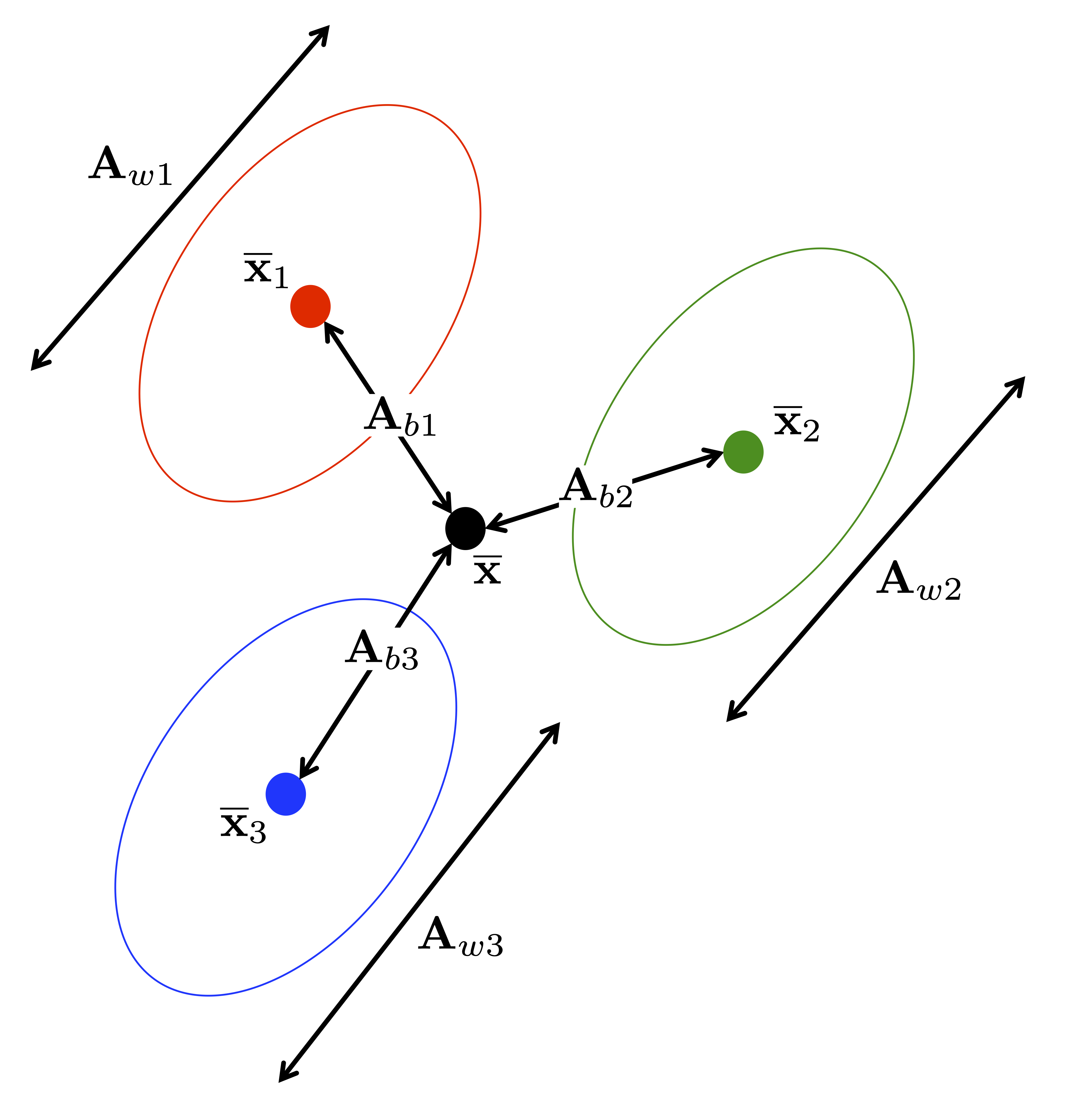
Fisher’s Criterion:
\[\max\dfrac{\text{between-group variability} (\textbf{A}_b)}{\text{within-group variability} (\textbf{A}_w)}\]
The following figure illustrates these different sources of variability in the case of three groups.
The new variables \(y_1,\ldots,y_{g-1}\) have by construction decreasing discrimination power. Normality and homogeneous group covariance matrices are typically assumed for \(x_1,\ldots,x_p\).
Discriminant analysis provides an optimum solution in the sense that it finds the linear combination of the original variables which maximises the ratio of between-group variation to within-group variation. The maximum number of canonical variates which can be derived is the smaller of (\(g-1\)) and \(p\). The scores from the canonical variates are uncorrelated with each other as in PCA.
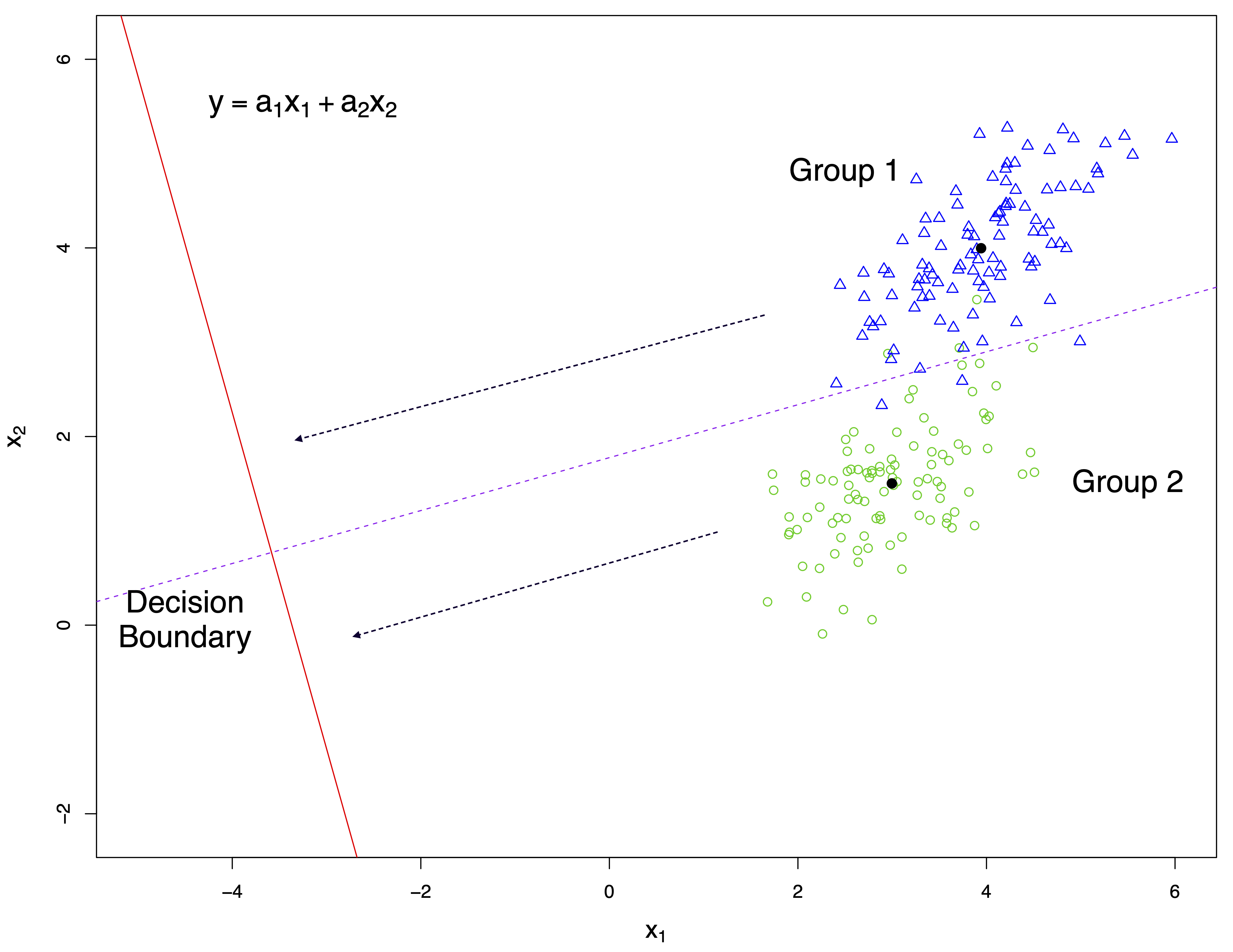
The following figure illustrates graphically the general idea of discriminant analysis for the case of two variables (\(x_1\), \(x_2\)) and two groups. Points and group centres are projected onto the discriminant score axis (red solid line). Samples are allocated to a group according to their closeness to the projected group centres. A threshold (decision boundary) is computed to determine group allocation.
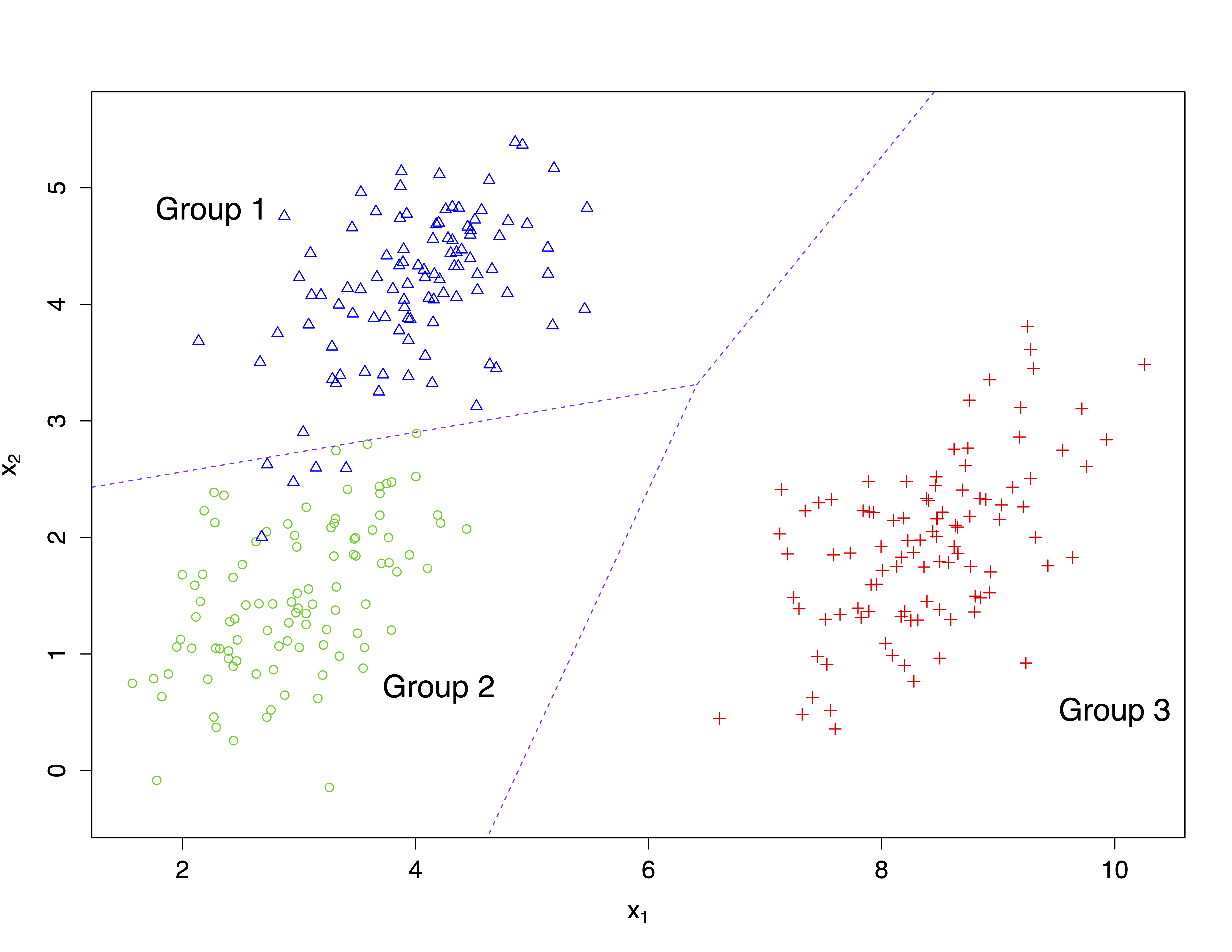
The following figure shows another example for the case of two variables \(x_1\) and \(x_2\) and three groups.
3.3 Discriminant analysis of the pea pods data set
The data consist of 40 pea pods: 11 each of varieties A, B, C and 7 of variety D were collected, and the length(mm), width(mm), curvature(mm) and greenness (intensity units) of each pod was recorded. Curvature is the minimum distance from an end-to-end straight line to the top edge of the pod. These variables will be used as classifiers or predictors.
'data.frame':   40 obs. of  5 variables:
 $ Variety  : Factor w/ 4 levels "A","B","C","D": 1 1 1 1 1 1 1 1 1 1 ...
 $ Length   : num  84.3 91 87.5 96.7 90.8 ...
 $ Width    : num  14.6 15.8 15.8 16.3 15.2 15.8 15.8 15.8 15.2 16.3 ...
 $ Curvature: num  1.4 1 0.6 1 1.4 1 1.1 1.2 1.5 1.2 ...
 $ Greenness: num  62.7 65.3 62.9 66.2 66.8 63.5 70.3 66.4 60 63.1 ...
We want to know if we can use our 4 variables to discriminate cleanly among the four varieties A, B, C and D. Clearly, from the graph below there is some scope to achieve this as the varieties can be distinguished based on some pairs of predictors, but it is not clear how best to proceed.
# Define colours for varieties A, B, C and D respectively
colours <- c("black", "red", "green", "blue")[pods$Variety]
# Show data in scatterplot matrix
pairs(pods[, 2:5], col = colours)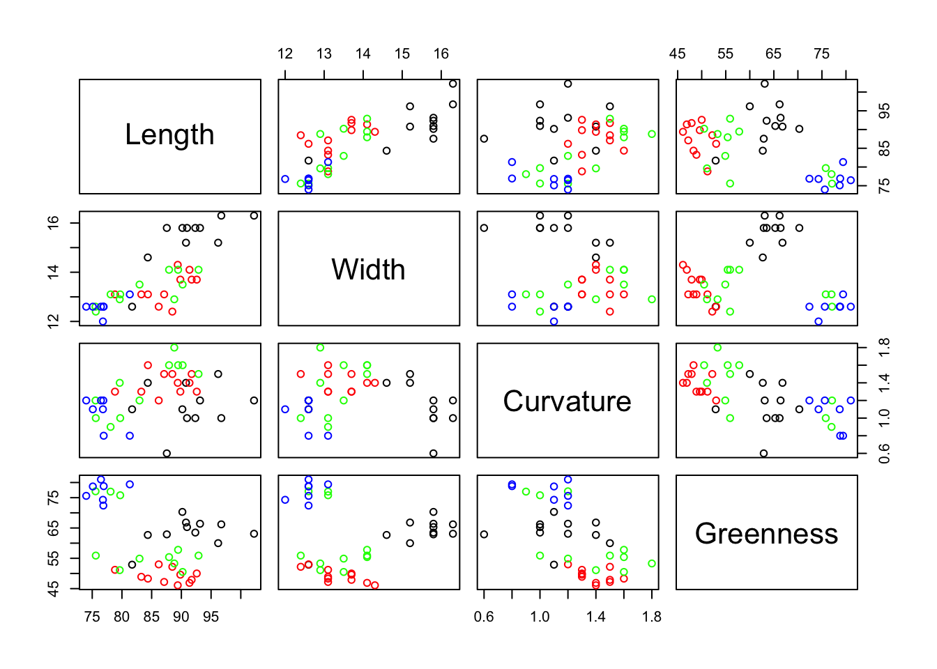
Linear discriminant analysis (LDA) is implemented in the lda function of the MASS package.
library(MASS)
pods.lda <- lda(Variety ~ Length + Width + Greenness + Curvature, data = pods)
pods.lda
Call:
lda(Variety ~ Length + Width + Greenness + Curvature, data = pods)
Prior probabilities of groups:
A B C D
0.275 0.275 0.275 0.175
Group means:
Length Width Greenness Curvature
A 91.46727 15.38182 63.64545 1.136364
B 87.55818 13.35455 49.20909 1.390909
C 83.71273 13.30000 60.42727 1.345455
D 76.78286 12.58571 77.17143 1.057143
Coefficients of linear discriminants:
LD1 LD2 LD3
Length 0.001652454 0.06000551 -0.20421720
Width -0.969487037 -1.24960352 1.05045155
Greenness 0.136886953 -0.09085738 0.01115272
Curvature 1.192856684 -0.07422961 5.18180976
Proportion of trace:
LD1 LD2 LD3
0.5644 0.4206 0.0150 The output from the function lda provides the group means, the “loadings” \(a_{ij}\) of the canonical variates (coefficients of linear discriminants), and their % discriminatory power (proportion of trace). The scores and other elements are also stored in the lda object. The first canonical variate contrasts Curvature with Width, while the second is essentially representing Width alone. In turn these account for 56.44% and 42.06% of the discriminatory power (hence, reaching 96% of the between group variability explained in total). The interpretation of the coefficients is conducted as for PCA (note also that the indeterminacy property holds here, so you might find instances were the coefficients appear multiplied by -1). One conclusion from this analysis might be that pod Length and pod Greenness do not vary according to Variety, at least not sufficiently to assist in Varietal identification.
The canonical variate loadings are generated directly from the function lda but the remaining useful information is obtained from the function predict, including the scores as shown above. This generates for each sample three results:
- $class: predicted group allocation.
- $posterior: the estimated probability of belonging to each group.
- $x: sample scores on each canonical variate.
The discriminant scores can be used to represent the observations in low dimensions as in the PCA biplot and explore the overall similarity between groups. The following code extract the scores for the first two canonical variates (LDA1 and LDA2) and plot them.
pods.scores <- predict(pods.lda, dimen = 2, method = "plug-in")
plot(pods.scores$x[, 1], pods.scores$x[, 2], col = colours, xlab = "LDA1", ylab = "LDA2")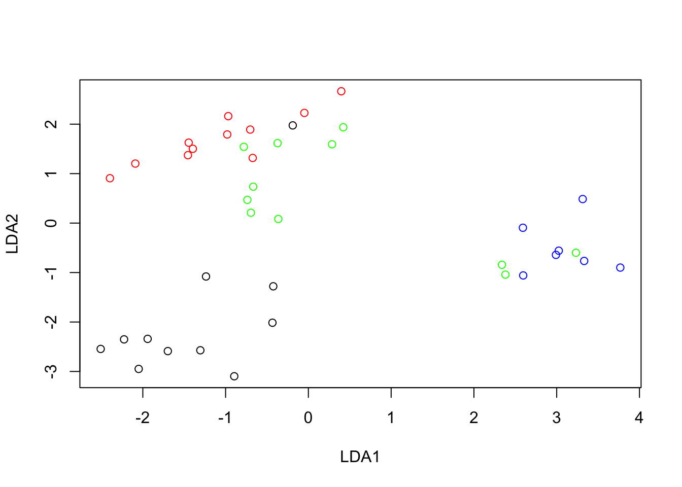
Variety D is the most distant from the others along the first canonical variate (LDA1), i.e. in terms of the contrast between Curvature and Width. It is interesting to observe that 3 samples of variety C (green) appear far from the others and very much mixed with the variety D samples. This is suggesting an error when registering the variety of those three samples. Variety A appears to be the most clearly distinguished as it is the least mixed with the others.
Note the section of the output referring to prior probabilities of groups. LDA uses these weights in its derivation of the canonical variates. The default weights are the relative frequencies of the factor levels, Variety in our case. This will be reasonable only if these frequencies reflect the true (usually unknown) relative frequencies of the levels of the factor we are trying to predict. However, when allocating a new sample to a group it is generally assumed that the new sample is equally likely to belong to each of the groups. Some discriminant analyses are very sensitive to the prior probabilities and you should always investigate the consequences of not using equal prior probabilities. If the groups are severely imbalanced, the performance is generally very biased against the smallest group.
With the pods data, the lower frequency of variety D has no implications for the likely variety of an unknown pod so we will change to equal prior probabilities.
pods.lda <- lda(Variety ~ Length + Width + Greenness + Curvature,
                data = pods, prior = c(.25, .25, .25, .25))
pods.lda
Call:
lda(Variety ~ Length + Width + Greenness + Curvature, data = pods,
prior = c(0.25, 0.25, 0.25, 0.25))
Prior probabilities of groups:
A B C D
0.25 0.25 0.25 0.25
Group means:
Length Width Greenness Curvature
A 91.46727 15.38182 63.64545 1.136364
B 87.55818 13.35455 49.20909 1.390909
C 83.71273 13.30000 60.42727 1.345455
D 76.78286 12.58571 77.17143 1.057143
Coefficients of linear discriminants:
LD1 LD2 LD3
Length 0.0001316129 -0.05938340 0.20440561
Width -0.8690751421 1.33236457 -1.03652090
Greenness 0.1445457201 0.07759319 -0.01425889
Curvature 1.0900541174 -0.05095316 -5.20468590
Proportion of trace:
LD1 LD2 LD3
0.6340 0.3528 0.0132 Equal prior probabilities have not changed the loadings very much, but the first canonical variate now has increased discriminatory power.
3.4 Prediction performance
The table below, occasionally called the confusion table, shows the classification performance of the canonical variates (using the first LDA model fit considering unequal prior probabilities). The rows show the “true” classifications, the columns show the predicted classifications. With perfect prediction all the off-diagonal elements of the table would be zero.
       A  B  C  D Sum
  A   10  1  0  0  11
  B    0 11  0  0  11
  C    0  3  5  3  11
  D    0  0  0  7   7
  Sum 10 15  5 10  40
The percentage of correctly classified samples provides the overall accuracy of 82.5%. Interpretation can be easier by using proportions (by rows in the table below).
             A          B          C          D
  A 0.90909091 0.09090909 0.00000000 0.00000000
  B 0.00000000 1.00000000 0.00000000 0.00000000
  C 0.00000000 0.27272727 0.45454545 0.27272727
  D 0.00000000 0.00000000 0.00000000 1.00000000
The predictions and performance above use the fitted model to classify the original samples into their known groups. This is helpful to have a crude assessment of prediction performance. This is the default re-substitution behaviour of predict using its argument method="plug-in" (see ?predict-lda for details). However, this type of prediction gives an over-optimistic assessment of the LDA classification (the same data are used to train the model and assess its performance). Ideally, we should use new samples (a validation or test data set) not used in building the LDA model. A statistical approach to resemble that is using cross-validation (see Resampling and Cross-Validation section below). The assessment of the performance of the model by cross-validation (CV) will be generally more realistic than those based on the same data used to fit the model (re-substitution). Different ways to perform cross-validation can be implemented. For example, with leave-one-out cross-validation, we leave out a sample, construct the LDA model and conduct prediction, then predict the class of the left-out sample. This is repeated for every sample in the data set. We can access to this cross-validation approach using the own lda function.
pods.lda.cv <- lda(Variety ~ Length + Width + Greenness + Curvature,
                   data = pods, prior = c(.25, .25, .25, .25), CV = T)
pods.lda.cv$class
[1] C A A A A A A A A A B C B B B B B B B B B B C B B B C B B B D D D D D D D D
[39] D D
Levels: A B C DThe associated confusion table is the following.
       A  B  C  D Sum
  A    9  1  1  0  11
  B    0 10  1  0  11
  C    0  6  2  3  11
  D    0  0  0  7   7
  Sum  9 17  4 10  40
The cross-validated overall accuracy is reduced to 70%.
             A          B          C          D
  A 0.81818182 0.09090909 0.09090909 0.00000000
  B 0.00000000 0.90909091 0.09090909 0.00000000
  C 0.00000000 0.54545455 0.18181818 0.27272727
  D 0.00000000 0.00000000 0.00000000 1.00000000
Note the poorer predictive performance suggested by these cross-validated calculations.
3.4.1 Class prediction for new (unknown) samples
We need to put the new samples into a data.frame. For illustration, suppose two new samples whose values are equal to those of the last two samples in the pea pods data file.
newdata <- rbind(c(73.99, 12.6, 1.2, 75.6), c(76.87, 12.6, 1.2, 72.4))
newdata <- data.frame(newdata)
# Create names for columns as in original data set
names(newdata) <- c("Length", "Width", "Curvature", "Greenness")
# Prediction
predict(pods.lda, newdata, dimen = 2)
$class
[1] D D
Levels: A B C D
$posterior
A B C D
1 3.010571e-05 2.002509e-05 0.02128692 0.9786630
2 9.522514e-05 2.932670e-04 0.09584560 0.9037659
$x
LD1 LD2
1 2.757671 0.2496968
2 2.295504 -0.1696256Both new samples have been allocated to variety D.
3.5 Case study: classification of bank notes
The data (Flury and Riedwyl, 1988) consist of six variables measured on 100 genuine and 100 counterfeit old Swiss bank notes. The first column contains the grouping variable (Genuine, Fake), the next ones correspond to the following 6 variables:
- Length: Length of the bank note.
- HeightL: Height of the bank note, measured on the left.
- HeightR: Height of the bank note, measured on the right.
- DistLB: Distance of inner frame to the lower border.
- DistUB: Distance of inner frame to the upper border.
- LengthD: Length of the diagonal.
Observations 1–100 are the genuine bank notes and the other 100 observations are the counterfeit bank notes. The aim is to study how these measurements may be used in determining whether a note is genuine or fake.
3.5.1 Preliminaries
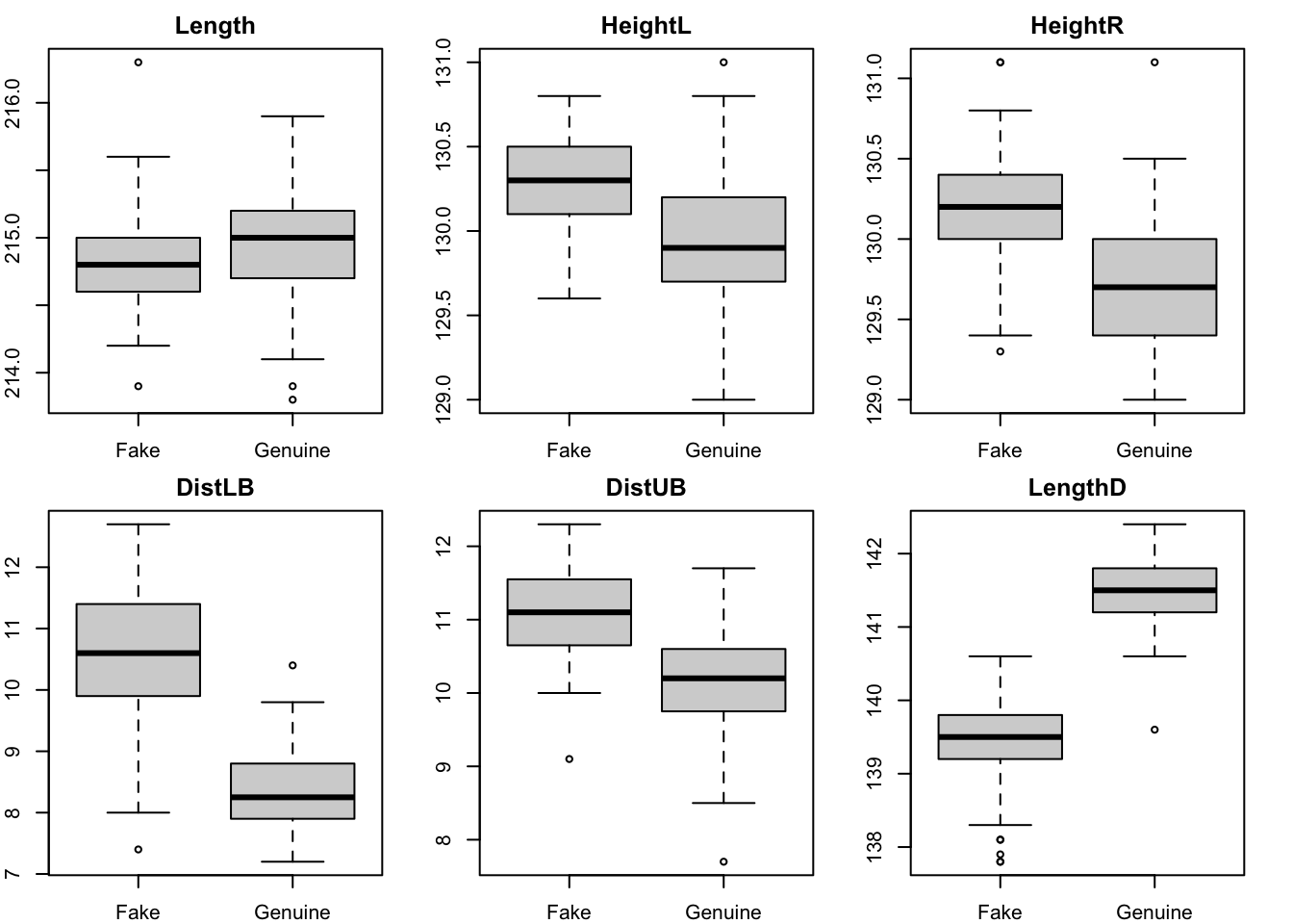
- Conduct exploratory inspection of the variables. What variables seem to be most helpful to distinguish groups?
Variables like LengthD and DistLB show the clearest differences between groups. Maybe Length will not be very helpful.
load("bank_notes.Rdata")
# Visual inspection by group
par(mfrow = c(2, 3)) # Boxplots arrangement
par(mar = c(2, 2, 2, 2))
for (i in 2:ncol(bank)) {
  boxplot(bank[, i] ~ Group, data = bank, main = names(bank)[i])
}
- Test for differences in mean between groups using multivariate analysis of variance (MANOVA). What does the result mean in relation to our aims?
# Compare group means
bank.manova <- manova(cbind(Length, HeightL, HeightR, DistLB, DistUB, LengthD) ~ Group,
                      data = bank)
summary(bank.manova, test = "Hotelling-Lawley")
Df Hotelling-Lawley approx F num Df den Df Pr(>F)
Group 1 12.184 391.92 6 193 < 2.2e-16 ***
Residuals 198
---
Signif. codes: 0 '***' 0.001 '**' 0.01 '*' 0.05 '.' 0.1 ' ' 1Using the MANOVA Hotelling-Lawley’s test we conclude highly statistically significant differences in means (\(p < 0.0001\)). Hence, the selected variables seem to be useful to discriminate between groups.
 Response Length :
             Df  Sum Sq Mean Sq F value   Pr(>F)
Group         1  1.0658 1.06580  7.7724 0.005822 **
Residuals   198 27.1510 0.13713
---
Signif. codes:  0 '***' 0.001 '**' 0.01 '*' 0.05 '.' 0.1 ' ' 1

 Response HeightL :
             Df  Sum Sq Mean Sq F value    Pr(>F)
Group         1  6.3725  6.3725   64.49 8.496e-14 ***
Residuals   198 19.5651  0.0988
---
Signif. codes:  0 '***' 0.001 '**' 0.01 '*' 0.05 '.' 0.1 ' ' 1

 Response HeightR :
             Df Sum Sq Mean Sq F value    Pr(>F)
Group         1 11.187 11.1865  103.96 < 2.2e-16 ***
Residuals   198 21.305  0.1076
---
Signif. codes:  0 '***' 0.001 '**' 0.01 '*' 0.05 '.' 0.1 ' ' 1

 Response DistLB :
             Df Sum Sq Mean Sq F value    Pr(>F)
Group         1 247.53 247.531  292.15 < 2.2e-16 ***
Residuals   198 167.76   0.847
---
Signif. codes:  0 '***' 0.001 '**' 0.01 '*' 0.05 '.' 0.1 ' ' 1

 Response DistUB :
             Df Sum Sq Mean Sq F value    Pr(>F)
Group         1 46.561  46.561  112.79 < 2.2e-16 ***
Residuals   198 81.739   0.413
---
Signif. codes:  0 '***' 0.001 '**' 0.01 '*' 0.05 '.' 0.1 ' ' 1

 Response LengthD :
             Df  Sum Sq Mean Sq F value    Pr(>F)
Group         1 213.624 213.624  836.07 < 2.2e-16 ***
Residuals   198  50.591   0.256
---
Signif. codes:  0 '***' 0.001 '**' 0.01 '*' 0.05 '.' 0.1 ' ' 1
All comparisons per variable conclude statistically significant differences in mean between groups.
- Using a biplot, can you identify any variable playing a leading role in distinguishing groups?
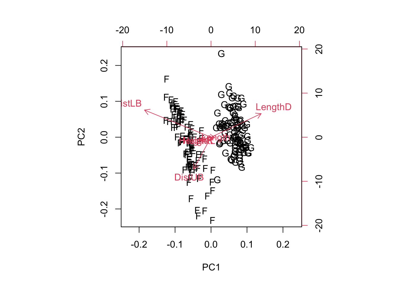
Groups are neatly distinguished along the LengthD axis.
3.5.2 Linear discriminant analysis
Note that the discriminant scores (also called canonical variates) are usually centred to have mean zero. The coefficients of the linear discriminant functions are shown in the output and given by the component scaling of a lda object. They are associated to centred variables. So the discriminant scores provided by lda are obtained multiplying them by the centred original data and not the original data directly. You can use str(bank.lda) to see all the components of a lda object or check the help system out (?lda).
- Perform LDA on the bank notes data and show the main results, including discriminant function coefficients, re-substitution and cross-validated confusion matrices.
library(MASS)
bank.lda <- lda(Group ~ ., data = bank) # Using formula interface: Group on all the others
bank.lda # Main output of the function.
Call:
lda(Group ~ ., data = bank)
Prior probabilities of groups:
Fake Genuine
0.5 0.5
Group means:
Length HeightL HeightR DistLB DistUB LengthD
Fake 214.823 130.300 130.193 10.530 11.133 139.450
Genuine 214.969 129.943 129.720 8.305 10.168 141.517
Coefficients of linear discriminants:
LD1
Length 0.005011113
HeightL 0.832432523
HeightR -0.848993093
DistLB -1.117335597
DistUB -1.178884468
LengthD 1.556520967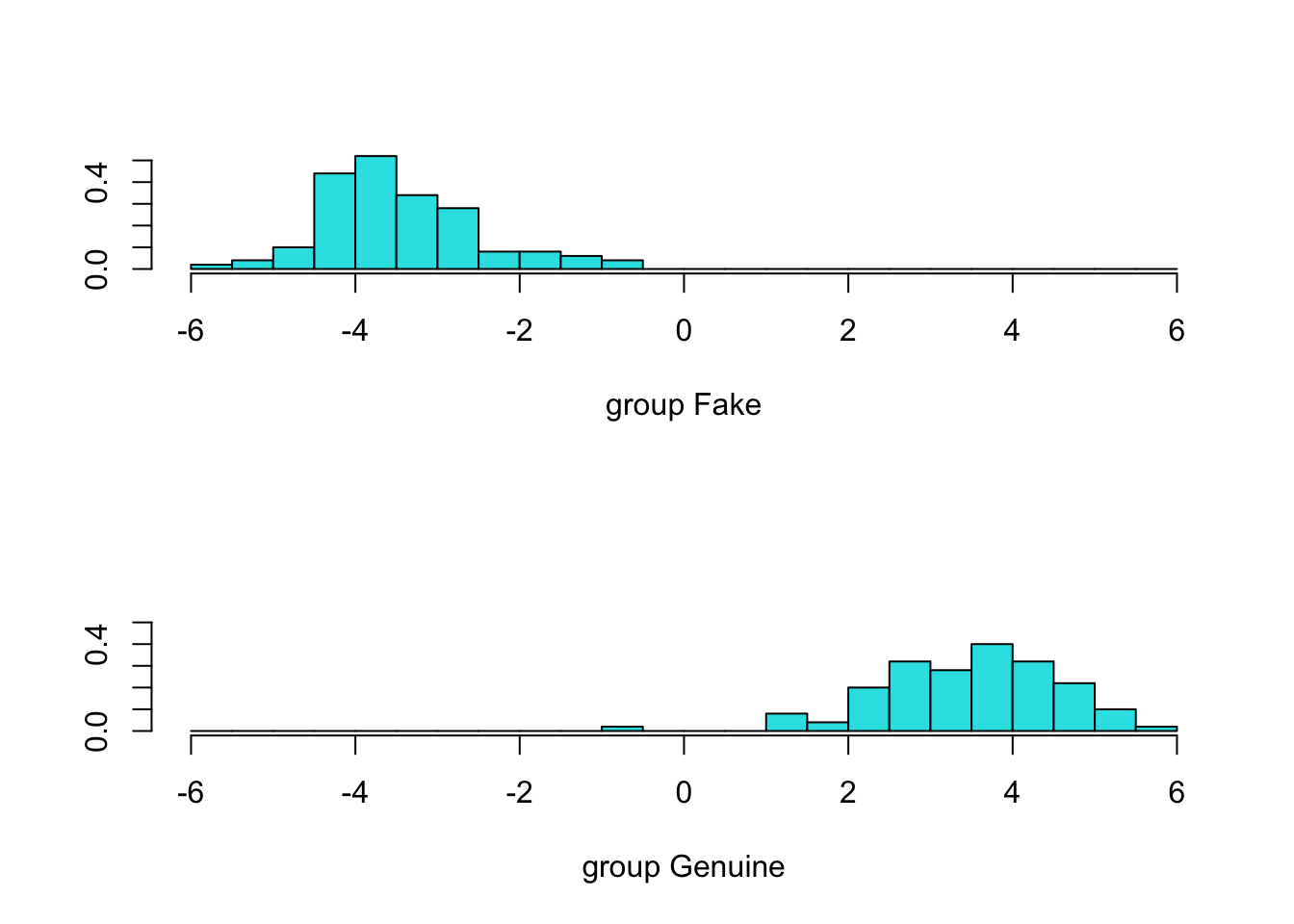
Predictions for each bank note (showing the first 6 only using the head function):
       LD1
1 2.150948
2 4.587317
3 4.578290
4 4.749580
5 4.213851
6 2.649422 Fake Genuine
1 3.245560e-07 0.9999997
2 1.450624e-14 1.0000000
3 1.544496e-14 1.0000000
4 4.699587e-15 1.0000000
5 1.941700e-13 1.0000000
6 1.017550e-08 1.0000000[1] Genuine Genuine Genuine Genuine Genuine Genuine
Levels: Fake Genuine# Confusion matrix based on re-substitution
# table(bank$Group, predict(bank.lda)$class)
# Maybe clearer editing the column names
pred.gr <- c("Predict Fake", "Predict Genuine")
table(bank$Group, factor(predict(bank.lda)$class, labels = pred.gr))
          Predict Fake Predict Genuine
  Fake             100               0
  Genuine            1              99
# Confusion matrix based on leave-one-out cross-validation
# (no difference with raw confusion matrix in this case)
bank.lda.cv <- lda(Group ~ ., data = bank, CV = T)
table(bank$Group, factor(bank.lda.cv$class, labels = pred.gr))
          Predict Fake Predict Genuine
  Fake             100               0
Genuine 1 99- Compute the correlation between discriminant scores and original variables as an approximation to their importance to distinguish the groups.
             Length    HeightL    HeightR     DistLB      DistUB    LengthD
Length   1.00000000  0.2312926  0.1517628 -0.1898009 -0.06132141  0.1943015
HeightL  0.23129257  1.0000000  0.7432628  0.4137810  0.36234960 -0.5032290
HeightR  0.15176280  0.7432628  1.0000000  0.4867577  0.40067021 -0.5164755
DistLB  -0.18980092  0.4137810  0.4867577  1.0000000  0.14185134 -0.6229827
DistUB  -0.06132141  0.3623496  0.4006702  0.1418513  1.00000000 -0.5940446
LengthD  0.19430146 -0.5032290 -0.5164755 -0.6229827 -0.59404464  1.0000000
LD1      0.20216804 -0.5156052 -0.6103648 -0.8030978 -0.62665368  0.9353514
               LD1
Length   0.2021680
HeightL -0.5156052
HeightR -0.6103648
DistLB  -0.8030978
DistUB  -0.6266537
LengthD  0.9353514
LD1      1.0000000
Focusing on the last line for the discriminant scores (LD1), we can see that the results are consistent with what we obtained before.
How to classify a new observation using the model?
# Classification of a new observation
new <- matrix(c(214.70, 131.12, 131.01, 10.63, 10.99, 140.13), ncol = 6) # New data
new <- as.data.frame(new) # Create data.frame ...
names(new) <- names(bank[, 2:7]) # ... with the same var names
predict(bank.lda, newdata = new) # Provides allocated group, posterior prob and score
$class
[1] Fake
Levels: Fake Genuine
$posterior
Fake Genuine
1 0.9999999 7.114744e-08
$x
LD1
1 -2.3694433.6 Resampling and cross-validation
Resampling methods involve repeatedly drawing samples from a data set and recompute statistics or refit models of interest on each sample in order to obtain additional information. Cross-validation (CV) is a statistical resampling method commonly used to obtain estimates of the performance of predictive models from the available data. These estimates are generally more realistic than those based on the observed data set only (re-substitution). A data set is split into a training data set used to fit models and estimate parameters and a validation data set that does not participate in the fitting process and is used to assess the performance of the model. Sometimes an additional completely independent is also used for further performance assessment. This is then called a test data set, but often validation and test data set are used exchangeably.
There are quite a few ways to perform cross-validation:
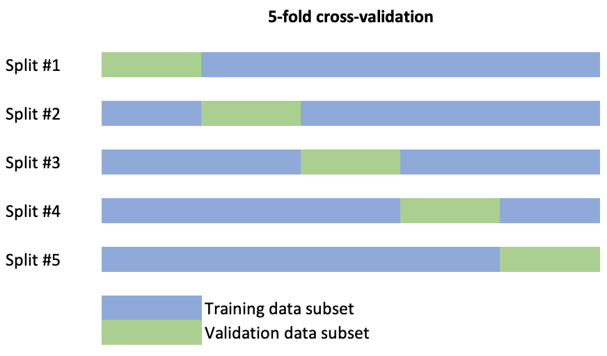
- K-fold cross-validation randomly divides the data into \(k\) blocks or splits of roughly equal size. Each of the blocks is left out in turn as validation data and the other \(k-1\) blocks are used to train the model. The held-out block is predicted and these predictions are summarised into some type of performance measure. For example accuracy (overall proportion of cases rightly allocated) in a classification problem or the mean squared error (MSE), \[MSE=\frac{1}{n}\sum_{i=1}^n(y_i-\hat{y}_i)^2,\] in a regression problem. When \(k\) is equal to the sample size this procedure is known as leave-one-out CV (LOOCV). A schematic display of the splits of a data set to conduct 5-fold cross-validation is the following.
Repeated \(k\)-fold CV does the same as above but more than once. For example, five repeats of 10-fold CV would give 50 total resamples. Note that this is not the same as 50-fold CV.
Leave Group Out cross-validation (LGOCV), also known as Monte Carlo CV, randomly leaves out some set percentage of the data a large number of times.
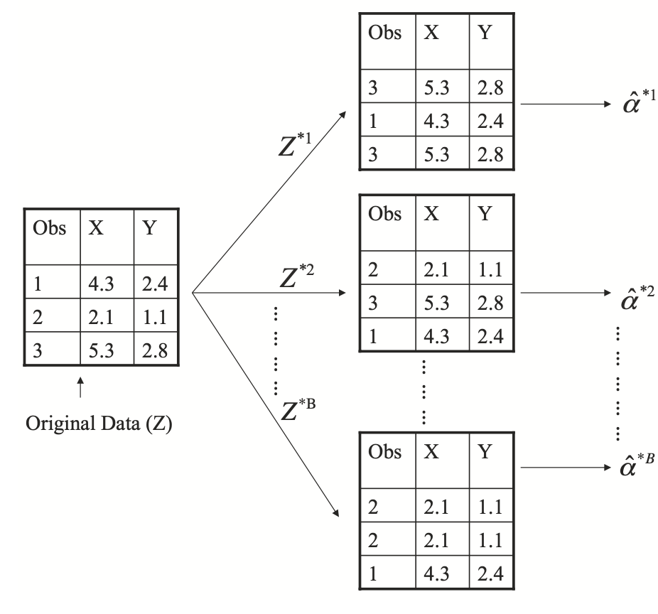
Bootstrap takes a random sample with replacement from the training set a large number of times. Since the sampling is with replacement, there is a strong likelihood that some training set samples will be represented more than once. As a consequence of this, some training set data points will not be contained in the bootstrap sample. The model is trained on the bootstrap sample and those data points not in that sample are predicted as hold-outs. Note that bootstrapping is actually generally used for statistical inference and data modelling for different purposes. The following figure illustrates the bootstrap procedure (extracted from James et al. (2021), An introduction to Statistical Learning, 2nd edition, Springer).
Which resampling or cross-validation method to use depends on the data set size and a some other factors. Each of the methods above can be characterised in terms of their bias and precision. This leads to what is called the bias-variance tradeoff, what is a recurring topic in statistical modelling and machine learning methods in general.
For example, when assessing the performance of a regression model we are interested in minimising the MSE, but MSE is decomposed as
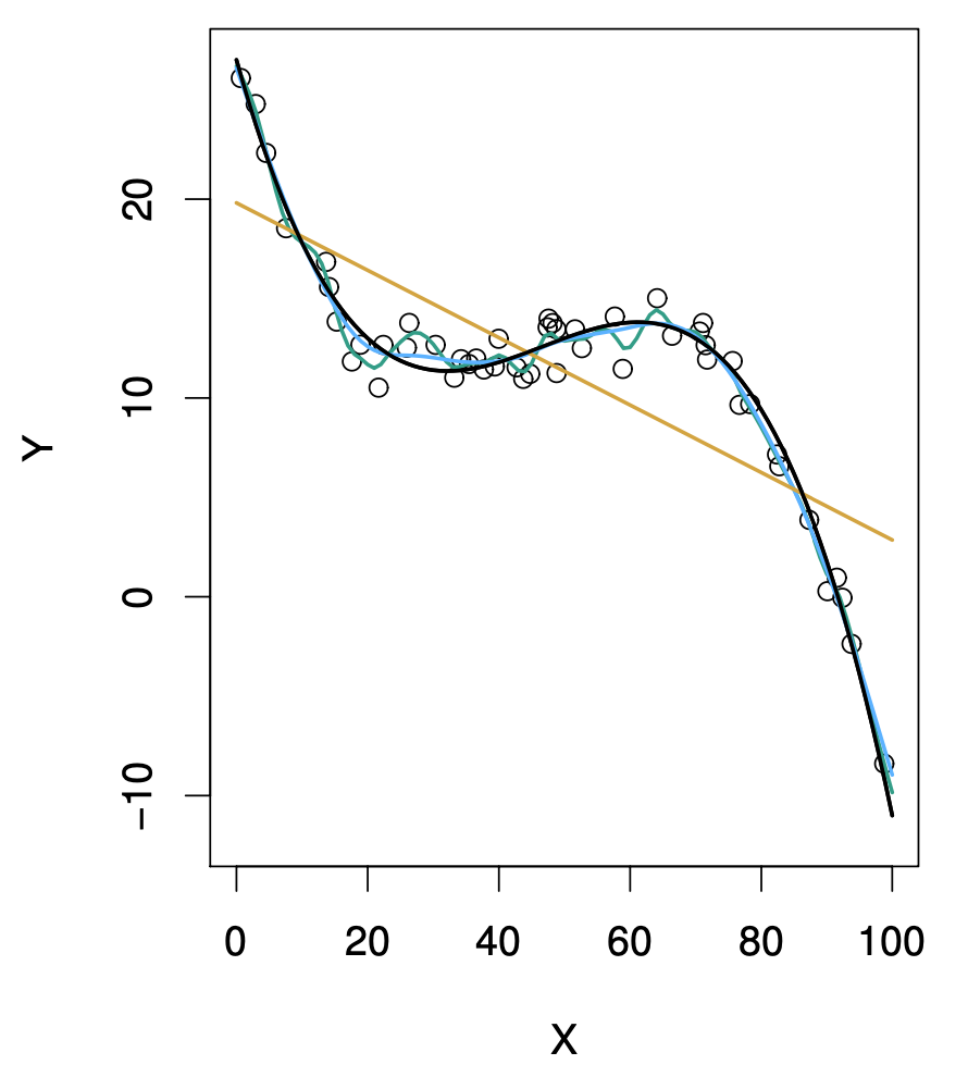
\[MSE = Bias(\hat{y},y)^2 + Var(\hat{y})\] Hence, in order to minimise MSE, a method should simultaneously achieve low bias and low variance. Bias refers to the error, the deviation of the estimate from the actual value. Variance refers to how variable the estimate is, the amount by which the estimate would change using a different training data set. Ideally the estimate should not vary too much using different training data sets. In general, more flexible statistical methods have higher variance. For example, in the following figure we show a set of observed data (empty circles) and two fits to them: a linear fit (orange curve; using linear regression; strict modelling of the relationship between \(Y\) and \(X\)) and a non-linear fit (dark curve; using a smoothing spline; flexible modelling of the relationship between \(Y\) and \(X\)) (from James et al., 2021).
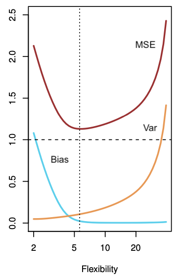
If the fit of the smoothing spline to the data is too tight, the bias will tend to be lower, but small changes in the training data can result in large changes in the estimates \(\hat{y}\). Hence, the variance in the estimates or predictions will tend to be higher. On the other hand, linear regression is obviously too simplistic for these data. Thus, regardless of the training data, the estimation bias will be high. However, if the data were closer to linear, given enough data, linear regression would produce accurate predictions. The tradeoff comes from the fact that as more flexible is a method the variance tends to increase and the bias tends to decrease. Initially, the bias typically decreases faster than the variance increases, then leading to decrease in MSE. However, at some point increasing flexibility has little impact on the bias and the variance starts to increase significantly, leading to increase in MSE. In both the regression and classification modelling settings, choosing the correct level of flexibility is critical to the success of any method. The following figure illustrates this from simulated data (adapted from James et al., 2021).
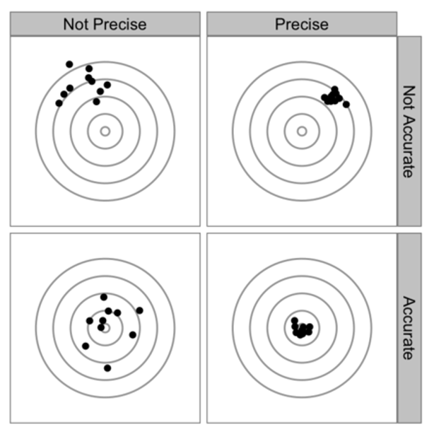
The bias-variance tradeoff is analogously present in the context of cross-validation. Some types of CV have higher bias than others and the same is true for variance. The following figure summarises the discussion about bias (accuracy) versus variance (precision). The lower right is obviously the best place.
The bias and variance of a CV procedure is thought to be related to how much data is held out. For example, with LOOCV we repeatedly fit the statistical method using training sets that contain \(n-1\) observations (nearly as many as in the entire data set). The MSE (computed from the validation or test set) is estimated as an average:
\[MSE_{CV}=\frac{1}{n}\sum_{i=1}^n MSE_i,\] where \(MSE_i\) is the MSE obtained in each round of the LOOCV procedure. LOOCV tends to have lower bias than other methods. But it can be computationally expensive to implement because the model has to be fit \(n\) times, especially if \(n\) is large and if each individual model is slow to fit. As said above, using \(k\)-fold CV we split the set of observations into \(k\) groups (folds) with one of then used as validation set and the remaining \(k-1\) as training set. This is computationally lighter than LOOCV as it is repeated \(k < n\) times (producing \(k\) estimates of MSE which are averaged at the end of the process). However another potential advantage is that \(k\)-fold CV often has less variance than LOOCV, since there is less overlap between training sets. With LOOCV we are averaging the outputs of \(n\) fitted models, each of which is trained on an almost identical set of observations; therefore, these outputs are highly (positively) correlated with each other. The mean of many highly correlated quantities has higher variance than does the mean of many quantities that are not as highly correlated. In exchange \(k\)-fold CV is expected to be more biased than LOOCV. If you hold-out 50% of your data using 2-fold CV, the thinking is that the final MSE estimate will be more biased than one that held out 10%. On the other hand, it is accepted that holding less data out (in the case of LOOCV just one sample) increases variance, since each hold-out sample has less data to get a stable estimate of performance. However, other factors are important. For example, if you have a ton of data, the bias and variance of 10- or even 5-fold CV may be acceptable. It has been shown empirically, that using \(k = 5\) or \(k = 10\) is a good compromise in general, yielding to errors that have neither excessively high bias nor very high variance (see also Kuhn and Johnson (2013), Applied Predictive Modeling, Springer for further discussion).
3.7 Exercises
- PEA PODS data. To what extent are the scores on the canonical axes correlated? Multiply one of the variables by 10 and redo the discriminant analysis. What effect has this rescaling had on the loadings, scores and posterior probabilities? A slick way of doing this is to use the R function
I(“Inhibit”), as follows.
pods.lda <- lda(Variety ~ Length + Width + I(10 * Greenness) + Curvature,
                data = pods, prior = c(.25, .25, .25, .25))
BRINE data. A set of geochemical measurements on brines from wells. Each sample is assigned to a stratigraphic unit, listed in the last column. How successfully can the geochemical measurements be used to predict stratigraphic unit?
PEA PODS data. Redo the discriminant analysis omitting the sample(s) you think might have been misclassified originally. Have the results changed in any way? To which variety does the discriminant analysis allocate the mis-classified sample(s)? To do this either create a copy of the data file and remove the sample(s) that seem to have been originally mis-classified or use the
subsetargument oflda.SKULLS data. Carry out a discriminant analysis of the skulls data but before doing so check to see what kind of distributions the original variables have. What is the maximum number of canonical variates that can be derived? How many are worth using to discriminate among the epochs? What is the predictive ability of the selected canonical variates?