Chapter 4 Correspondence analysis
4.1 Introduction
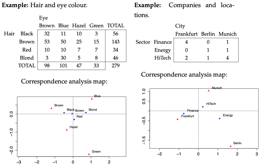
Correspondence analysis (CA) is a multivariate tool for analysing the associations between rows and columns of contingency tables, or tabular data in general. A contingency table is a two-way frequency table where the joint frequencies of two categorical variables are reported. The well-known test for independence, based on the \(\chi^2\) (chi-square) statistic, is useful to investigate statistically significant association. However there are no simple ways for detecting which parts of the table are responsible for this association. CA is one tool that allows to see the pattern of association in the data and to generate hypotheses that can be tested in a subsequent stage of research.
CA reduces the dimension of a contingency table in order to obtain a graphical representation of rows and columns in a low-dimensional space. The idea is to extract new dimensions (axis) in decreasing order of importance so that the main information of the table can be summarised in spaces with low dimensions. For example, if only two axis are used, the results can be shown on a two-dimensional plane. This is why CA is considered as a PCA for categorical variables. With PCA, the total variance is partitioned into independent contributions from the principal components. CA, instead, decomposes a measure of association, particularly the \(\chi^2\) statistic. Another difference is that CA works on count/frequency data, whereas PCA is thought for continuous data. Actually, CA can work on any non-negative discrete data as long as they are measured on the same scale, so that it makes sense to compute row sums and column sums.
Hence, the variables of interest can also be discrete quantitative variables, such as the number of family members or the number of accidents an insurance company had to cover during one year, etc. Here, each possible value that the variable can have defines a row or a column category. Of course this will be practically feasible as long as the number of different values observed is low-moderate. Continuous variables may be taken into account by discretisation, i.e. defining categories in terms of intervals or classes of values which the variable can take on. Thus contingency tables can be used in many situations, implying that correspondence analysis is a very useful tool in many applications.
4.2 Basic elements
Let \(\mathbf N\) denote the \(I\times J\) contingency table with entries \(n_{ij}\) and positive row and column sums. The matrix \(\mathbf N\) can be converted to the matrix correspondence matrix \(\mathbf P=[p_{ij}]\) by dividing \(\mathbf N\) by the grand total \(n=\sum_{i=1}^I\sum_{j=1}^Jn_{ij}\). The vectors of marginal relative frequencies by rows and columns are called row and column masses with components
\[r_i=\sum_{j=1}^Jp_{ij}\quad\mbox{and}\quad c_j=\sum_{i=1}^Ip_{ij}\]
All these quantities \(\mathbf P\), \(\mathbf r=(r_1,\ldots,r_I)\) and \(\mathbf c=(c_1,\ldots,c_J)\) are proportions adding up to 1 in each case. Besides, the row and column profiles are defined as the row (column) frequencies divided by their row (column) total. There is a complete symmetry in CA analysis in that the results are the same regardless of the main interest being on the rows or on the columns of the table.
The well-known Pearson’s \(\chi^2\) test for independence measures the discrepancy between all the observed, \(n_{ij}\), and expected, \(e_{ij}=nr_ic_j\), frequencies for each cell \((i,j)\) of the table using the \(\chi^2\) statistic:
\[\chi^2=\sum_{i=1}^I\sum_{j=1}^J\frac{(n_{ij}-e_{ij})^2}{e_{ij}}=n\sum_{i=1}^I\sum_{j=1}^J\frac{(p_{ij}-r_ic_j)^2}{r_ic_j}\]
which has distribution \(\chi^2_{(I-1)(J-1)}\) under independence. The larger this value, the more discrepant the observed and expected frequencies are, i.e., the less convincing the assumption of independence of rows and columns is.
The quantity \(\chi^2/n\), called total inertia or simply inertia, plays a central role in CA as a measure of variation in a data table. This is equivalent to the total variability in PCA.
We seek to represent the row categories by scores which approximate the distances/similarities between the row profiles of the table and scores for the columns which approximate the distances/similarities between the columns of the table, both after a little scaling and aiming to maximise the explained data variability (total inertia). These scores are given by the set of first dimensions for the rows and columns of the CA solution, as for PCA.
We can proceed to generate second dimensions for the rows and columns in a manner similar to the way in which a second principal component is derived in PCA. And so on for further dimensions, each dimension describing less of the association between the rows and columns than the previous dimensions.
Typically, we plot the row and column scores for the first two dimensions in the same plot to produce a CA biplot or map.
4.3 CA of the moths data set
The moths data set shows the counts of 12 different moth species recorded in light traps at 14 sites throughout the UK. For each site we also have its Northing, Easting and Type (Woodland, Farmland, Parkland).
   Site   E   N Type  M1  M2 M3  M4  M5 M6  M7  M8  M9 M10 M11 M12
1     A 513 213    W 154  51  0  37  20 55   1   5   1 724   0   0
2     B 465 164    W  34  57  5  66   8 21 141  33  35  84   0   0
3     C 480 143    W   5  26  5  30   2 20  12  66 214  73   0   2
4     D 418 107    W   0  37 55   5   3 63   7  23   6   0   0   0
5     E 306 138    P  31 109  6  12  23 56   9 403  58   0   2  13
6     F 282  45    F   1  40  1  79  66 35  77  35   6   0   0   0
7     G 263 284    F   5  14  2  27 144 54  24   7   7   2   0  14
8     H 520 280    P   3  17  0 316  79 19  21   4  48   7   0   0
9     I 575 266    F   0   7  0 126  37 10 101  83   3   0   0   0
10    J 363 594    W  64 383  1   0  47  0   0   0   0  79  65   0
11    K 260 756    P  26 373  2   0 228  0   0   0   0 129 393   0
12    L 237 809    W   8 306 94   2 108  0   0   7   0   0  55   0
13    M 316 864    W   6 141  0   6  38  0   9   0   0   0  10   0
14    N 263 874    W   9 535  0   0 156  0   0   0   0 429 141   6
# Extract the counts and use site as row label
counts <- data.frame(row.names = moths$Site, moths[5:16])The following computes the CA solution using the R package ca (the function corresp in the MASS package is an alternative, although it has less options). The output provides, amongst others, information about the amount of explained variability by the successive CA dimensions (so-called principal inertias, technically corresponding to eigenvalues) and the scores for rows and columns, i.e. their coordinates in the low-dimensional representation. The first two dimensions explain 47.9% of the total variability/inertia.
 Principal inertias (eigenvalues):
           1        2        3        4      5        6        7
Value      0.604647 0.377591 0.349915 0.2102 0.186407 0.111768 0.100981
Percentage 29.5%    18.42%   17.07%   10.26% 9.1%     5.45%    4.93%
           8        9        10       11
Value      0.066095 0.023946 0.016025 0.001933
Percentage 3.22%    1.17%    0.78%    0.09%


 Rows:
             A       B       C     D      E      F      G      H      I       J
Mass     0.126  0.0584  0.0549 0.024 0.0871 0.0410 0.0362  0.062 0.0443  0.0771
ChiDist  1.484  1.2371  2.0952 2.356 1.8430 1.2140 1.6048  1.976 1.6400  0.9585
Inertia  0.279  0.0894  0.2411 0.133 0.2960 0.0605 0.0933  0.242 0.1191  0.0709
Dim. 1  -0.601  0.8334  1.3013 0.564 1.3059 1.0849 0.4967  1.483 1.6599 -0.8795
Dim. 2  -2.192 -0.5295 -0.7443 1.117 0.5151 0.3490 0.6063 -0.112 0.1929  0.3665
             K      L       M       N
Mass     0.139  0.070  0.0253  0.1540
ChiDist  1.134  1.338  1.0771  0.7718
Inertia  0.179  0.125  0.0294  0.0917
Dim. 1  -0.967 -0.665 -0.6080 -0.8787
Dim. 2   0.793  1.444  0.9772 -0.1612


 Columns:
             M1     M2      M3      M4      M5      M6      M7     M8      M9
Mass     0.0418  0.253  0.0206  0.0852  0.1158  0.0402  0.0485 0.0804  0.0456
ChiDist  1.1587  0.802  2.7702  1.8725  0.8636  1.4941  1.9031 1.9738  2.3538
Inertia  0.0561  0.163  0.1584  0.2988  0.0863  0.0897  0.1757 0.3132  0.2528
Dim. 1  -0.3998 -0.709 -0.1035  1.5703 -0.1920  0.8832  1.3980 1.6030  1.6069
Dim. 2  -1.3178  0.689  1.8790 -0.1958  0.7470 -0.0125 -0.0242 0.4834 -0.6108
           M10     M11     M12
Mass     0.184  0.0804 0.00422
ChiDist  1.212  1.4239 2.29173
Inertia  0.271  0.1630 0.02219
Dim. 1  -0.699 -1.1606 0.78124
Dim. 2 -1.730 0.9842 0.59183 Dim1 Dim2
A -0.601 -2.192
B 0.833 -0.529
C 1.301 -0.744
D 0.564 1.117
E 1.306 0.515
F 1.085 0.349
G 0.497 0.606
H 1.483 -0.112
I 1.660 0.193
J -0.879 0.367
K -0.967 0.793
L -0.665 1.444
M -0.608 0.977
N -0.879 -0.161 Dim1 Dim2
M1 -0.400 -1.3178
M2 -0.709 0.6891
M3 -0.103 1.8790
M4 1.570 -0.1958
M5 -0.192 0.7470
M6 0.883 -0.0125
M7 1.398 -0.0242
M8 1.603 0.4834
M9 1.607 -0.6108
M10 -0.699 -1.7297
M11 -1.161 0.9842
M12 0.781 0.5918The CA map (which is a biplot as it represents two sets of points, rows and column coordinates) is not particularly revealing.
But labelling the sites by their Northing reveals that the first dimension is mainly a north/south axis and that species 2 and 11 do well at these northerly sites.
# Re-label sites using Northing
rownames(counts) <- moths$N
moths.ca2 <- ca(counts)
plot(moths.ca2, main = "Sites labelled by Northing")
In general, when both the Site and Species scores sit close to each other and far from the origin this implies they have a strong association. The count for that species on that site is greater than you would expect if there was no association. For example, species 2 and 11 in the CA plot sit close to sites J, K, L and M. This is because those species have particularly high (negative) scores at those sites which themselves have high (negative) scores, both in the first dimension. The same is true, but with positive scores, for Species 4 and 7 at sites H and I.
A CA map is interpreted as follows:
Proximity of two row (or two column) scores indicates similar, proportional row (column) profiles across columns (across rows).
Proximity between rows and column scores reflects on positive association between them, and the opposite implies negative association.
If all row and column scores are very close to the origin, this implies poor association between them (typically obtaining a no statistically significant result from a \(\chi^2\)-test of independence).
The origin \((0,0)\) represents the average of the row and column profiles. Hence, a particular point projected close to the origin indicates closeness to the average profile.
All the interpretations must be carried out in view of the quality of the representation, which is given by the cumulated variability/inertia explained by the two first principal axes/CA dimensions.
We have used above what is formally called a symmetric CA map, but there are some (asymmetric) variants (essentially modifications of the axis scaling) which may more precisely represent relationships between rows and columns. See e.g. Greenacre (2007) “Correspondence Analysis in Practice” for more details.
4.4 Case study 1: funding and disciplines
The data set consists of a cross-classification table in which counts from \(N=796\) scientific researchers were distributed according to their scientific discipline (geology, biochemistry, chemistry, zoology, physics, engineering, microbiology, botany, statistics and mathematics) and funding category (A, B, C, D, E). A to D are the categories for researchers who are receiving research grants, from A (most funded) to D (least funded), while E is a category assigned to researchers whose grant applications were not successful (source: Greenacre, 2007).
4.4.1 Contingency table, profiles, masses
      A  B  C  D  E
Geol  3 19 39 14 10
Bioc  1  2 13  1 12
Chem  6 25 49 21 29
Zool  3 15 41 35 26
Phys 10 22 47  9 26
Engi  3 11 25 15 34
Micr  1  6 14  5 11
Bota  0 12 34 17 23
Stat  2  5 11  4  7
Math 2 11 37 8 20 A B C D E Sum
Geol 0.004 0.024 0.049 0.018 0.013 0.107
Bioc 0.001 0.003 0.016 0.001 0.015 0.036
Chem 0.008 0.031 0.062 0.026 0.036 0.163
Zool 0.004 0.019 0.052 0.044 0.033 0.151
Phys 0.013 0.028 0.059 0.011 0.033 0.143
Engi 0.004 0.014 0.031 0.019 0.043 0.111
Micr 0.001 0.008 0.018 0.006 0.014 0.046
Bota 0.000 0.015 0.043 0.021 0.029 0.108
Stat 0.003 0.006 0.014 0.005 0.009 0.036
Math 0.003 0.014 0.046 0.010 0.025 0.098
Sum 0.039 0.161 0.389 0.162 0.249 1.000 A B C D E
Geol 0.035 0.224 0.459 0.165 0.118
Bioc 0.034 0.069 0.448 0.034 0.414
Chem 0.046 0.192 0.377 0.162 0.223
Zool 0.025 0.125 0.342 0.292 0.217
Phys 0.088 0.193 0.412 0.079 0.228
Engi 0.034 0.125 0.284 0.170 0.386
Micr 0.027 0.162 0.378 0.135 0.297
Bota 0.000 0.140 0.395 0.198 0.267
Stat 0.069 0.172 0.379 0.138 0.241
Math 0.026 0.141 0.474 0.103 0.256 A B C D E
Geol 0.097 0.148 0.126 0.109 0.051
Bioc 0.032 0.016 0.042 0.008 0.061
Chem 0.194 0.195 0.158 0.163 0.146
Zool 0.097 0.117 0.132 0.271 0.131
Phys 0.323 0.172 0.152 0.070 0.131
Engi 0.097 0.086 0.081 0.116 0.172
Micr 0.032 0.047 0.045 0.039 0.056
Bota 0.000 0.094 0.110 0.132 0.116
Stat 0.065 0.039 0.035 0.031 0.035
Math 0.065 0.086 0.119 0.062 0.1014.4.2 Correspondence analysis
We focus on the row profiles; that is, the main interest is on research areas and their relationship with the funding categories. Note that the ca function also admits the data.frame as input directly. That is, no need to create a table object first
Looking at the relative position of the research categories, we can see that the first axis (horizontal) lines up the four categories of funding in their intrinsic ordering, from D (less funding) to A (most funding). The second axis, is a contrast between E (no funding) against the others. Hence, the more a discipline is low down in the map the less funding is granted. The more to the right, the more the funding received. The best place to be would be the top right quadrant. Physics is the most to the right, it shows the highest percentage of type A researchers (8.8%, see row profiles table). But it is at the middle vertically since it has a percentage of non-funded researchers close to average (22.8% compared to 24.9%, see row profiles and masses in correspondence matrix above). Biochemistry is the discipline with the highest number of rejections in relative terms. Note that statements about the funding profiles of the disciplines must all be in relative terms. For absolute differences one should refer to the original data.
Geology, statistics, mathematics and biochemistry are all at a similar position on the first axis, but widely different on the second. This means that the researchers in these fields whose grants have been accepted have similar positions with respect to the funded categories A to D categories, but geology has much fewer rejections than biochemistry.
4.4.3 Decomposition of the inertia
Principal inertias (eigenvalues):

 dim    value      %   cum%   scree plot
 1      0.039117  47.2  47.2  ************
 2      0.030381  36.7  83.9  *********
 3      0.010869  13.1  97.0  ***
 4      0.002512   3.0 100.0  *
        -------- -----
 Total: 0.082879 100.0


Rows:
     name   mass  qlt  inr    k=1 cor ctr    k=2 cor ctr
1  | Geol |  107  916  137 |   76  55  16 |  303 861 322 |
2  | Bioc |   36  881  119 |  180 119  30 | -455 762 248 |
3  | Chem |  163  644   21 |   38 134   6 |   73 510  29 |
4  | Zool |  151  929  230 | -327 846 413 |  102  83  52 |
5  | Phys |  143  886  196 |  316 880 365 |   27   6   3 |
6  | Engi |  111  870  152 | -117 121  39 | -292 749 310 |
7  | Micr |   46  680   10 |   13   9   0 | -110 671  18 |
8  | Bota |  108  654   67 | -179 625  88 |  -39  29   5 |
9  | Stat |   36  561   12 |  125 554  14 |   14   7   0 |
10 | Math |   98  319   56 |  107 240  29 |  -61  79  12 |

Columns:
    name   mass  qlt  inr    k=1 cor ctr    k=2 cor ctr
1 |    A |   39  587  187 |  478 574 228 |   72  13   7 |
2 |    B |  161  816  110 |  127 286  67 |  173 531 159 |
3 |    C |  389  465   94 |   83 341  68 |   50 124  32 |
4 |    D |  162  968  347 | -390 859 632 |  139 109 103 |
5 |    E |  249  990  262 |  -32  12   6 | -292 978 699 |
The first part of the output of summary shows that the \(10\times 5\) table produces 4 principal axes (dimensions). The two first (used in the CA map) explain 83.9% of the total inertia. The value of the \(\chi^2\) statistic is \(total\;inertia\times n = 65.97.\)
The subsequent output provides more comprehensive details about how the inertia/variability is decomposed by rows and columns, the contributions of these to each principal axis, and how well they are represented in the CA map (we refer to Greenacre (2007)’s book for more details about these measures).
4.5 Case study 2: marine species abundance
The data set consists of abundance (frequencies) of 92 marine species in 13 stations (samples) in the North sea
species <- read.table("SpecAbund.txt", h = T, stringsAsFactors = TRUE)
# Show first lines of the table
head(species)
Species S4 S8 S9 S12 S13 S14 S15 S18 S19 S23 S24 R40 R42
1 Myri_ocul 193 79 150 72 141 302 114 136 267 271 992 5 12
2 Chae_seto 34 4 247 19 52 250 331 12 125 37 12 8 3
3 Amph_falc 49 58 66 47 78 92 113 38 96 76 37 0 5
4 Myse_bide 30 11 36 65 35 37 21 3 20 156 12 58 43
5 Goni_macu 35 39 41 37 32 45 41 41 31 29 64 32 23
6 Amph_fili 19 39 11 38 18 20 11 22 30 40 3 55 65Stations starting with S are close to oil-drill platform (pollution), stations R40 and R42 are regarded as clean reference samples.
# Extract the counts and use site as row label
sp.counts <- data.frame(row.names = species$Species, species[2:14])
sp.ca <- ca(sp.counts)
plot(sp.ca, map = "rowprincipal") # Use different scaling to facilitate interpretation
Stations form a curve from most polluted stations to least polluted stations. Reference clean stations (R40, R42) are far from the drilling area.
Station 24 separates out from the others: higher relative abundance of Echi.sp and Myri.ocul. here. Species Eumi.oke. is linked to the most polluted stations.
The two first CA dimensions explain 57.5% of the total variation.