Chapter 9 Multiple linear regression
9.1 Fitting the model
Instead of simple regression models of the form \(Y = a + bX + \epsilon\) we now consider several independent \(X\) variables
\[Y = b_0 + b_1X_1 + \ldots + b_pX_p + \epsilon\] Again the residual errors represented by \(\epsilon\) are assumed to be independent and normally distributed with mean 0 and constant variance \(\sigma^2\). Alternatively, we can say that \(Y\sim N(\mu,\sigma^2)\) where \(\mu = b_0 + b_1X_1 + \ldots + b_pX_p\).
We illustrate multiple regression using the savings data from the R package faraway.
'data.frame':   50 obs. of  5 variables:
 $ sr   : num  11.43 12.07 13.17 5.75 12.88 ...
 $ pop15: num  29.4 23.3 23.8 41.9 42.2 ...
 $ pop75: num  2.87 4.41 4.43 1.67 0.83 2.85 1.34 0.67 1.06 1.14 ...
 $ dpi  : num  2330 1508 2108 189 728 ...
 $ ddpi : num  2.87 3.93 3.82 0.22 4.56 2.43 2.67 6.51 3.08 2.8 ...
These data are savings rates, sr, for 50 countries, averaged across 1960-70. The variable dpi is disposable, per-capita income in US dollars; ddpi is the % rate of change in per capita disposable income, sr is aggregate personal saving divided by disposable income. The pop15 and pop75 columns are the percentages of the population under 15 and over 75.
As always, before carrying out a regression analysis, some plotting and calculation of summary statistics should be done to familiarise yourself with the data and to identify unexpected or odd features. We can do pairwise scatterplots of variables from the savings data set.
The correlation matrix quantifies the extent of the linearity in these pairwise plots.
         sr  pop15  pop75   dpi   ddpi
sr     1.00 -0.456  0.317  0.22  0.305
pop15 -0.46  1.000 -0.908 -0.76 -0.048
pop75  0.32 -0.908  1.000  0.79  0.025
dpi    0.22 -0.756  0.787  1.00 -0.129
ddpi 0.30 -0.048 0.025 -0.13 1.000Note that sr is not highly correlated with any one of the other variables but these other variables do have some high correlations among themselves. Now we can proceed with the regression analysis.
Call:
lm(formula = sr ~ pop15 + pop75 + dpi + ddpi, data = savings)

Residuals:
    Min      1Q  Median      3Q     Max
-8.2422 -2.6857 -0.2488  2.4280  9.7509

Coefficients:
              Estimate Std. Error t value Pr(>|t|)
(Intercept) 28.5660865  7.3545161   3.884 0.000334 ***
pop15       -0.4611931  0.1446422  -3.189 0.002603 **
pop75       -1.6914977  1.0835989  -1.561 0.125530
dpi         -0.0003369  0.0009311  -0.362 0.719173
ddpi         0.4096949  0.1961971   2.088 0.042471 *
---
Signif. codes:  0 '***' 0.001 '**' 0.01 '*' 0.05 '.' 0.1 ' ' 1

Residual standard error: 3.803 on 45 degrees of freedom
Multiple R-squared:  0.3385,    Adjusted R-squared:  0.2797
F-statistic: 5.756 on 4 and 45 DF,  p-value: 0.0007904
The fitted regression is
\[sr = 28.6 - 0.46 pop15 - 1.69 pop75 - 0.0003dpi + 0.41ddpi\]
The interpretation of the regression coefficients in multiple regression is identical to the interpretation for simple regression. For example sr decreases by 1.69 for every increase of size 1 in pop75. Again, the intercept, 28.6, is the value of sr when all the independent variables are zero (a situation which cannot occur in practice).
We begin by asking whether it is worth having all four \(X\) variables in the model; in other words whether \(b_1 = b_2 = b_3 = b_4 = 0\). This is assessed by the \(F\) test statistic at the end of the summary output (\(F=5.756\)) that has associated a very small p-value \(p = 0.0007904\). Thus, the probability of obtaining an \(F\) ratio (signal to noise) as extreme as 5.7 when all the regression coefficients are zero is \(p=0.0008\). This is so unlikely that we conclude that at least one of the coefficients is not zero.
The model assumes that the residual term \(\epsilon\) has a normal distribution with mean zero and an (unknown) variance \(\sigma^2\). The residual standard error in the results, 3.803, is the estimate of \(\sigma\).
The significance levels for each term in the regression, Pr(>|t|), test the null hypothesis that this term is zero (i.e. the coefficient \(b_i=0\)), given that all the other terms are already in the model. It is important to distinguish between testing whether \(X_i\) affects \(Y\) (which we would do by simple linear regression), and whether \(X_i\) affects \(Y\) after all the other \(X\) variables have been included in the model. The results above test the latter hypothesis. And, as said, we can interpret the regression coefficient \(b_i\) as the amount \(Y\) will increase when \(X_i\) increases by 1.
Multiple R-squared and Adjusted R-squared are measures of goodness of fit. The closer to 1 these are, the better the fit. There tends to be a larger discrepancy between these two measures in the context of multiple regression than simple regression. Adjusted R-squared is the preferred measure because it takes into account the number of \(X\) variables that have been fitted. With the unadjusted multiple R-squared, the more variables you include the more R-squared approaches 1.
All other results from the lm function are interpreted in the same way as for simple linear regression and we can generate the same plots and access the same information as before.
oldpar <- par()
# Modify them to do a 2x2 matrix of graphs
par(oma = c(0, 0, 0, 0), mfrow=c(2, 2))
plot(m.sr.1)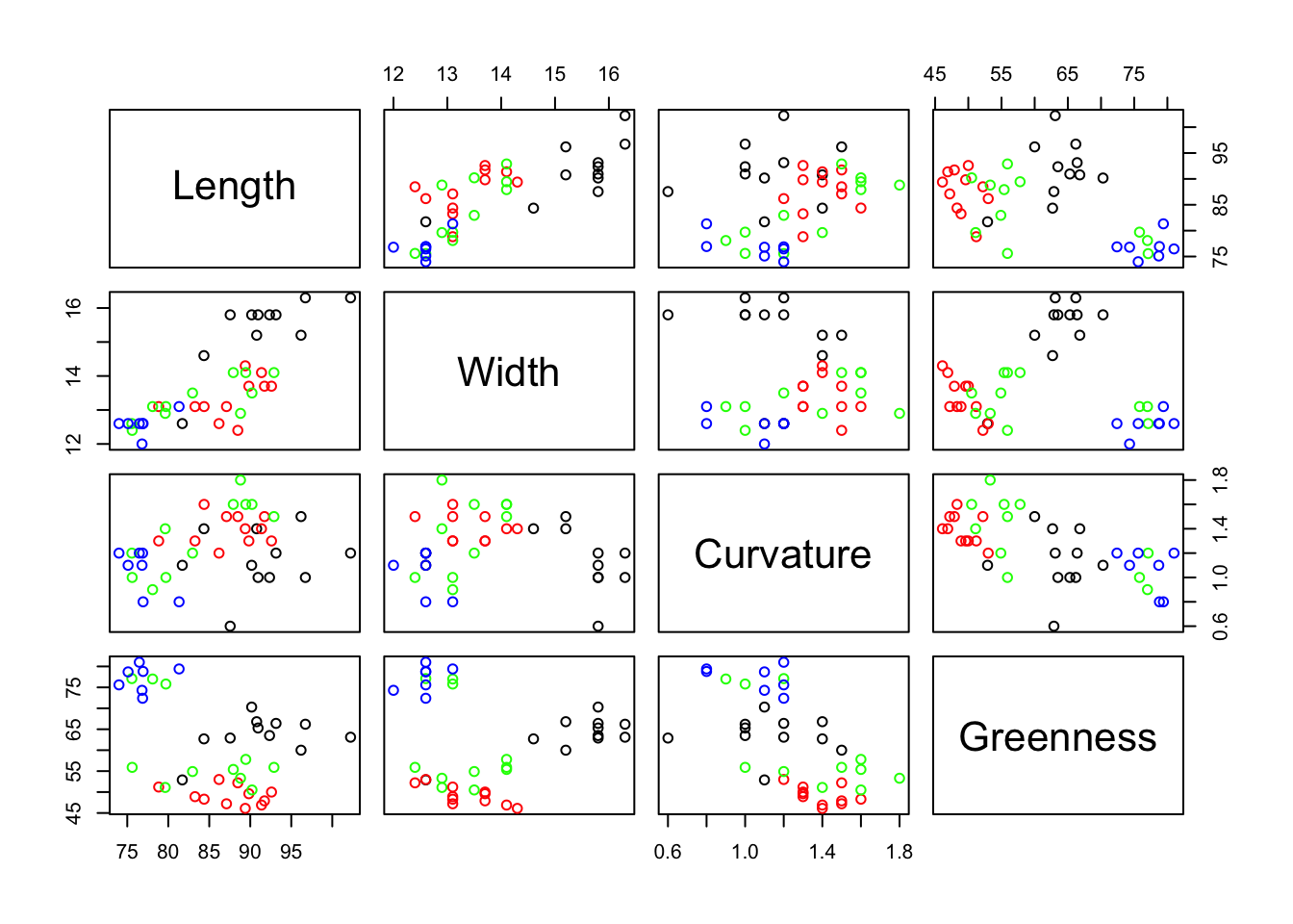
We can equally obtain confidence intervals for the parameter estimates
                   0.5 %      99.5 %
(Intercept)  8.785490197 48.34668288
pop15       -0.850220708 -0.07216559
pop75       -4.605929128  1.22293377
dpi         -0.002841194  0.00216739
ddpi        -0.117993927  0.93738378
To predict savings rates for new combinations of pop15, pop75, dpi and ddpi we must put these new levels into a data.frame object.
newvalues <- data.frame(pop15=c(32,33), pop75=c(3,2), dpi <- c(700,700),ddpi=c(3,3))
ci <- predict(m.sr.1,newvalues,interval="confidence")
pi <- predict(m.sr.1,newvalues,interval="prediction")
The confidence interval tells us about the average value of sr. The prediction interval tells us about a single value of sr. Notice how the prediction interval is much wider than the confidence interval.
9.2 Testing subsets of the \(X\) variables
We can test a wide range of hypotheses on the explanatory variables such as:
- Is it worth including any \(X\) variables in the model?
- Could \(X_3\) reasonably be dropped from the model?
- Could \(X_2\) and \(X_3\) be dropped simultaneously from the model without loss?
- Do \(X_1\) and \(X_4\) have the same coefficients?
- Is it reasonable to force the coefficient of one of the \(X\)’s to be 1?
The first of these is the \(F\)-test we have already met. All of these example hypotheses have one feature in common: they can all be expressed as a null hypothesis which is a subset of an alternative Hypothesis full model.
Thus, for the second example,
\[H_0: mean(Y) = b_0 + b_1X_1 + b_2X_2 + \;\;\; + b_4X_4\] \[H_A: mean(Y) = b_0 + b_1X_1 + b_2X_2 + b_3X_3 + b_4X_4\] Or \(H_0\) could also be written as
\[H_0: b_3 = 0\] For the third example,
\[H_0: mean(Y) = b_0 + b_1X_1 + \;\;\;\;\;\; + b_4X_4\] \[H_A: mean(Y) = b_0 + b_1X_1 + b_2X_2 + b_3X_3 + b_4X_4\] Or \[H_0: b_2 = b_3 = 0\] The test statistic for hypothesis comparisons of this type is based on the residual sums of squares (RSS). For any regression we have actual observations \(Y\), fitted (estimated) observations \(\hat{Y}\) and the residuals \((Y-\hat{Y})\). The RSS \(\sum (Y-\hat{Y})^2\) is a measure of how well the fitted model matches the data, low values indicate a good fit.
When \(H_0\) is true the RSS of the submodel (\(H_0\)) and the RSS of the full Model (\(H_A\)) should be approximately the same. However when \(H_0\) is false we would expect the RSS of the submodel to be noticeably greater than the RSS of the full model. So large values of \(RSS(sub) - RSS (full)\) will suggest that the \(H_0\) is false. The test statistic is
\[F=\frac{(RSS(sub)-RSS(full))/(p-q)}{RSS(full)/(n-1-p)},\] where \(n\) is the number of observations, \(p\) is the number of terms in the full model and \(q\) is the number of terms in the submodel.
When \(H_0\) is true this test statistic has an \(F\) distribution with \((p-q)\) and \((n-1-p)\) degrees of freedom. Large values of the test statistic are evidence away from the null hypothesis towards the alternative hypothesis.
Returning to the savings data set, we will test whether it is worth having dpi in the model. That is, we are going to test
\[H_0: b_3 = 0\] \[H_A: b_3 \neq 0\]
Ho <- lm(sr~ pop15+pop75+ddpi, data=savings)
Ha <- lm(sr~pop15+pop75+dpi+ddpi, data=savings)
anova(Ho,Ha)
Analysis of Variance Table
Model 1: sr ~ pop15 + pop75 + ddpi
Model 2: sr ~ pop15 + pop75 + dpi + ddpi
Res.Df RSS Df Sum of Sq F Pr(>F)
1 46 652.61
2 45 650.71 1 1.8932 0.1309 0.7192The test statistic in this case is
\[F=\frac{(652.61-650.71) / (4-3)}{650.71 / (50-1-4)}\] and
[1] 0.720119The result is not statistically significant at the usual \(5\%\) significance level. The data are not suggesting to reject the null hypothesis and hence we conclude that dpi has no additional effect on savings when the effects of pop15, pop75 and ddpi are already taken into account.
Note that we had already seen this result.
Call:
lm(formula = sr ~ pop15 + pop75 + dpi + ddpi, data = savings)

Residuals:
    Min      1Q  Median      3Q     Max
-8.2422 -2.6857 -0.2488  2.4280  9.7509

Coefficients:
              Estimate Std. Error t value Pr(>|t|)
(Intercept) 28.5660865  7.3545161   3.884 0.000334 ***
pop15       -0.4611931  0.1446422  -3.189 0.002603 **
pop75       -1.6914977  1.0835989  -1.561 0.125530
dpi         -0.0003369  0.0009311  -0.362 0.719173
ddpi         0.4096949  0.1961971   2.088 0.042471 *
---
Signif. codes:  0 '***' 0.001 '**' 0.01 '*' 0.05 '.' 0.1 ' ' 1

Residual standard error: 3.803 on 45 degrees of freedom
Multiple R-squared:  0.3385,    Adjusted R-squared:  0.2797
F-statistic: 5.756 on 4 and 45 DF,  p-value: 0.0007904
The significance of the additional effect of dpi using a \(t\)-test is based on a p-value equal to 0.7192, nearly numerically identical to that from the approach above using a \(F\)-test. In this particular circumstance, and only in this circumstance, when the numerator degrees of freedom is 1, the \(F\) statistic is the same as the squared \(t\) statistic and generates the same p-value.
9.3 ANOVA summary of multiple regression
Often the results of a regression analysis are presented in an ANOVA table format, as follows.
Analysis of Variance Table

Response: sr
          Df Sum Sq Mean Sq F value    Pr(>F)
pop15      1 204.12 204.118 14.1157 0.0004922 ***
pop75      1  53.34  53.343  3.6889 0.0611255 .
dpi        1  12.40  12.401  0.8576 0.3593551
ddpi       1  63.05  63.054  4.3605 0.0424711 *
Residuals 45 650.71  14.460
---
Signif. codes:  0 '***' 0.001 '**' 0.01 '*' 0.05 '.' 0.1 ' ' 1
The first line of the anova table shows the results of testing
\[H_0: mean(Y) = b_0\] \[H_A: mean(Y) = b_0 + b_1X_1\] and shows that \(X_1\) (pop15) explains significantly more of the savings ratio than using only the mean of the savings ratio (\(b_0\)).
The second line of the table shows the results of testing \[H_0: mean(Y) = b_0 + b_1X_1\] \[H_A: mean(Y) = b_0 + b_1X_1 + b_2X_2\] and shows that \(X_2\) (Pop75) just fails, at \(5\%\) significance level, to add significant improvement to the prediction of the savings ratio when \(X_1\) is already in the model.
The third line of the table shows the results of testing \[H_0: mean(Y) = b_0 + b_1X_1 + b_2X_2\] \[H_A: mean(Y) = b_0 + b_1X_1 + b_2X_2 + b_3X_3\] and shows that \(X_3\) (dpi) adds nothing to the prediction of the savings ratio when \(X_1\) and \(X_2\) are already in the model.
Finally the fourth line of the table shows the results of testing
\[H_0: mean(Y) = b_0 + b_1X_1 + b_2X_2 + b_3X_3\] \[H_A: mean(Y) = b_0 + b_1X_1 + b_2X_2 + b_3X_3 + b_4X_4\] and shows that \(X_4\) (ddpi) makes a significant improvement to the prediction of the savings ratio when \(X_1\), \(X_2\) and \(X_3\) are already in the model.
Thus the anova shows the cumulative effect of adding variables to the regression model. Variables are added in the order specified in the lm function.
It is important to be aware of the difference between this summary of the lm fit provided by the anova function and what is provided by the function summary applied on the lm object directly. The latter shows the results of testing each variable after all the others have been included in the model, i.e additional and not cumulative effects.
9.4 Variable/model selection strategies
Sometimes, when there are several variables for potential inclusion in the model, we wish to adopt a formal procedure for selecting the best subset.
There are varied proposals to do this and it is an active area of research. It is important to check the details of the options implemented by the software package used.
Examples of common procedures are:
- Backward elimination
- Forward selection
- Stepwise regression
- All subsets
With backward elimination we start with all the predictors in the model, then repeatedly remove the predictor with the highest \(p\)-value greater than some appropriate, pre-defined cut-off.
Forward selection reverses this approach and starts with no terms in the model. The single term with the smallest \(p\)-value beyond the cut-off is added first. Among the remaining variables the one with the strongest \(p\)-value beyond the cut-off, when added to the model, is selected. And so on. For this type of procedure the cut-off is usually less stringent than \(5\%\) and can be as high as \(20\%\).
Stepwise regression is a combination of the first two approaches and allows the possibility at each step of adding or dropping a variable, whichever has the strongest effect on the \(F\)-ratio. Best practice suggests starting both with no terms and with the full model to verify that both starting points lead to the same final model.
Criteria other than the \(F\)-ratio significance level can be used to accept or reject variables. Common alternatives are the Akaike Information Criterion (AIC) and the Bayesian Information Criterion (BIC). Both AIC and BIC criteria are based on various assumptions and asymptotic approximations. They are typically used together in model selection. The lower the value in these measures the better.
The AIC has a built in penalty for models with larger number of parameters. The AICc variant is recommended when sample size is small with respect to the number of model parameters. For nested models, estimates of relative importance of predictor variables can be made by summing the Akaike weights (evidence in favor of model \(i\) being the actual best model amongst a number of candidate models) of variables across all the models where the variables occur. The main difference in practice between AIC and BIC is the size of the penalty, BIC penalises model complexity more heavily. Thus, AIC always has a chance of choosing too big a model, regardless of the number of observations. BIC has very little chance of choosing too big a model if the number of observations is sufficient, but it has a larger chance than AIC, for any given number of observations, of choosing too small a model.
Another way to compare model specifications statistically is based on the likelihood ratio test (LRT; but limited to comparisons between two models at a time). The LR is a measure of the strength of evidence favouring a model (hypothesis) A over a model (hypothesis) B. In R, functions like anova and drop1 show results from AIC, BIC and LRT together.
Some software allows to search among all possible models to see which subset of variables fits the data best. This approach might take a lot of computing time and it is susceptible to presenting a best model which is not amenable to scientific interpretation. A modification of the all subsets method is often used when models are to be used for predictive (rather than explanatory) purposes. The fit of the model is assessed according to some predefined criterion (often the AIC or BIC). It requires that subsets are restricted to those which make scientific sense. Often several models have information criteria similar to the best model and the average of all the models within a certain distance of the best information criterion is used (see literature about multimodel inference and model averaging; Kenneth P. Burnham, David R. Anderson (2002). Model selection and multimodel inference: A practical information-theoretic approach. New York: Springer). The R package MuMIn implements methods for variable and multi-model selection within this framework.
No matter which model is selected as the best by any of the above strategies, its residuals should always be examined by the usual diagnostic plots to ensure the usual regression assumptions hold.
We illustrate an approach to backward elimination using the state data set. This data set comes with R and help(state) provides a full description. It is a collection of statistics from 50 US states: per capita income, illiteracy, life expectancy, murder and non-negligent manslaughter rate per 100000 population, percent high school graduates, mean number of days with min temperature less than 32F, and land area. The question of interest is whether we can predict life expectancy from the other variables.
data(state) #load a data set
statedata <- data.frame(state.x77, row.names=state.abb, check.names=TRUE)
# Model Life.Exp using ALL the variables in the data set
m.be1 <- lm(Life.Exp ~ . , data=statedata)
summary(m.be1)
Call:
lm(formula = Life.Exp ~ ., data = statedata)

Residuals:
     Min       1Q   Median       3Q      Max
-1.48895 -0.51232 -0.02747  0.57002  1.49447

Coefficients:
              Estimate Std. Error t value Pr(>|t|)
(Intercept)  7.094e+01  1.748e+00  40.586  < 2e-16 ***
Population   5.180e-05  2.919e-05   1.775   0.0832 .
Income      -2.180e-05  2.444e-04  -0.089   0.9293
Illiteracy   3.382e-02  3.663e-01   0.092   0.9269
Murder      -3.011e-01  4.662e-02  -6.459 8.68e-08 ***
HS.Grad      4.893e-02  2.332e-02   2.098   0.0420 *
Frost       -5.735e-03  3.143e-03  -1.825   0.0752 .
Area        -7.383e-08  1.668e-06  -0.044   0.9649
---
Signif. codes:  0 '***' 0.001 '**' 0.01 '*' 0.05 '.' 0.1 ' ' 1

Residual standard error: 0.7448 on 42 degrees of freedom
Multiple R-squared:  0.7362,    Adjusted R-squared:  0.6922
F-statistic: 16.74 on 7 and 42 DF,  p-value: 2.534e-10
Area has the largest \(p\)-value so we begin by eliminating it.
Call:
lm(formula = Life.Exp ~ Population + Income + Illiteracy + Murder +
    HS.Grad + Frost, data = statedata)

Residuals:
     Min       1Q   Median       3Q      Max
-1.49047 -0.52533 -0.02546  0.57160  1.50374

Coefficients:
              Estimate Std. Error t value Pr(>|t|)
(Intercept)  7.099e+01  1.387e+00  51.165  < 2e-16 ***
Population   5.188e-05  2.879e-05   1.802   0.0785 .
Income      -2.444e-05  2.343e-04  -0.104   0.9174
Illiteracy   2.846e-02  3.416e-01   0.083   0.9340
Murder      -3.018e-01  4.334e-02  -6.963 1.45e-08 ***
HS.Grad      4.847e-02  2.067e-02   2.345   0.0237 *
Frost       -5.776e-03  2.970e-03  -1.945   0.0584 .
---
Signif. codes:  0 '***' 0.001 '**' 0.01 '*' 0.05 '.' 0.1 ' ' 1

Residual standard error: 0.7361 on 43 degrees of freedom
Multiple R-squared:  0.7361,    Adjusted R-squared:  0.6993
F-statistic: 19.99 on 6 and 43 DF,  p-value: 5.362e-11
The adjusted \(R^2\) has hardly changed so eliminating Area has not given us a poorer fit. We next remove Illiteracy.
Call:
lm(formula = Life.Exp ~ Population + Income + Murder + HS.Grad +
    Frost, data = statedata)

Residuals:
    Min      1Q  Median      3Q     Max
-1.4892 -0.5122 -0.0329  0.5645  1.5166

Coefficients:
              Estimate Std. Error t value Pr(>|t|)
(Intercept)  7.107e+01  1.029e+00  69.067  < 2e-16 ***
Population   5.115e-05  2.709e-05   1.888   0.0657 .
Income      -2.477e-05  2.316e-04  -0.107   0.9153
Murder      -3.000e-01  3.704e-02  -8.099 2.91e-10 ***
HS.Grad      4.776e-02  1.859e-02   2.569   0.0137 *
Frost       -5.910e-03  2.468e-03  -2.395   0.0210 *
---
Signif. codes:  0 '***' 0.001 '**' 0.01 '*' 0.05 '.' 0.1 ' ' 1

Residual standard error: 0.7277 on 44 degrees of freedom
Multiple R-squared:  0.7361,    Adjusted R-squared:  0.7061
F-statistic: 24.55 on 5 and 44 DF,  p-value: 1.019e-11
The adjusted \(R^2\) has now improved slightly despite dropping Illiteracy. Income is next to go.
Call:
lm(formula = Life.Exp ~ Population + Murder + HS.Grad + Frost,
    data = statedata)

Residuals:
     Min       1Q   Median       3Q      Max
-1.47095 -0.53464 -0.03701  0.57621  1.50683

Coefficients:
              Estimate Std. Error t value Pr(>|t|)
(Intercept)  7.103e+01  9.529e-01  74.542  < 2e-16 ***
Population   5.014e-05  2.512e-05   1.996  0.05201 .
Murder      -3.001e-01  3.661e-02  -8.199 1.77e-10 ***
HS.Grad      4.658e-02  1.483e-02   3.142  0.00297 **
Frost       -5.943e-03  2.421e-03  -2.455  0.01802 *
---
Signif. codes:  0 '***' 0.001 '**' 0.01 '*' 0.05 '.' 0.1 ' ' 1

Residual standard error: 0.7197 on 45 degrees of freedom
Multiple R-squared:  0.736, Adjusted R-squared:  0.7126
F-statistic: 31.37 on 4 and 45 DF,  p-value: 1.696e-12
Note how the adjusted \(R^2\) has improved again. It is not obvious whether Population should be removed.
We have used a selection criterion based on significance levels. There are other criteria we might have used, for example improvement in adjusted \(R^2\). As said above, a popular criterion is AIC.
\[AIC = n\ln(RSS/n) + 2p\] We want to minimise the AIC. The AIC assesses a model by its RSS, accounting for the number of observations \(n\) and adding a penalty equal to twice the number of fitted parameters, \(p\). The AIC is good for comparing regression models. However, as a measure in its own right it does not tell us anything directly about the current model being fitted, i.e. how good it is in itself, the criteria just allows to compare its relative merit compared to others, but they might be all poor models. The adjusted \(R^2\) on the other hand, does tell us about the current model being fitted, the closer to 1 the better the fit.
The function step performs forward selection, backward elimination or stepwise regression automatically, using AIC rather than \(p\)-values. We illustrate backwards elimination below.
Start:  AIC=-22.18
Life.Exp ~ Population + Income + Illiteracy + Murder + HS.Grad +
    Frost + Area

             Df Sum of Sq    RSS     AIC
- Area        1    0.0011 23.298 -24.182
- Income      1    0.0044 23.302 -24.175
- Illiteracy  1    0.0047 23.302 -24.174
<none>                    23.297 -22.185
- Population  1    1.7472 25.044 -20.569
- Frost       1    1.8466 25.144 -20.371
- HS.Grad     1    2.4413 25.738 -19.202
- Murder      1   23.1411 46.438  10.305

Step:  AIC=-24.18
Life.Exp ~ Population + Income + Illiteracy + Murder + HS.Grad +
    Frost

             Df Sum of Sq    RSS     AIC
- Illiteracy  1    0.0038 23.302 -26.174
- Income      1    0.0059 23.304 -26.170
<none>                    23.298 -24.182
- Population  1    1.7599 25.058 -22.541
- Frost       1    2.0488 25.347 -21.968
- HS.Grad     1    2.9804 26.279 -20.163
- Murder      1   26.2721 49.570  11.569

Step:  AIC=-26.17
Life.Exp ~ Population + Income + Murder + HS.Grad + Frost

             Df Sum of Sq    RSS     AIC
- Income      1     0.006 23.308 -28.161
<none>                    23.302 -26.174
- Population  1     1.887 25.189 -24.280
- Frost       1     3.037 26.339 -22.048
- HS.Grad     1     3.495 26.797 -21.187
- Murder      1    34.739 58.041  17.456

Step:  AIC=-28.16
Life.Exp ~ Population + Murder + HS.Grad + Frost

             Df Sum of Sq    RSS     AIC
<none>                    23.308 -28.161
- Population  1     2.064 25.372 -25.920
- Frost       1     3.122 26.430 -23.877
- HS.Grad     1     5.112 28.420 -20.246
- Murder      1    34.816 58.124  15.528
Call:
lm(formula = Life.Exp ~ Population + Murder + HS.Grad + Frost,
    data = statedata)

Coefficients:
(Intercept)   Population       Murder      HS.Grad        Frost
  7.103e+01    5.014e-05   -3.001e-01    4.658e-02   -5.943e-03
At the start stage we see that the full model has \(AIC = -22.185\). The model with Area removed has \(AIC = -24.182\), an improvement. The model with Population removed has \(AIC = -20.560\), which is not as good as the full model. And so on. Removing Area generates the best value for AIC and leads to the subsequent step. This continues while there is an improvement. In this case the sequence of variable removals is very similar to our previous analysis using \(p\)-values rather than AIC.
9.5 Exercises
Using the savings data from Faraway’s book, multiply the variable dpi by 10. What changes does this produce in the regression results? Do these changes make sense?
The hills data set from the R library MASS shows the record times taken to race to the top of 35 hills, along with the race distance and total height climbed. Plot the data and derive the correlations among these variables. Derive the linear regression of time as a function of distance and height. Is this a good model? Using this model, how much extra time is added to the record for every 100 additional feet in height?
The gala data from Faraway records the number of species of tortoise on the various Galapagos islands. There are 30 islands. Endemics is the number of endemic species, Elevation is the highest point in metres on the island, Nearest is the distance (km) from the nearest island, Scrux is the distance (m) from Santa Cruz and Adjacent is the area of the adjacent island. Fit a regression model to predict the number of species on an island as a function of all the other variables. Do we need all the other variables? Is your model a good fit? Derive confidence and prediction intervals for the number of species when Endemics and all the other independent variables have values equal to their mean. What is the difference in interpretation for these two intervals?
Using the savings data from Faraway’s book investigate whether it is worth having ddpi in the model when dpi, Pop15 and Pop75 are already included. Use the same hypothesis testing procedure as the notes used for dpi and confirm your result against the
lmoutput for the model which includes all four \(X\) variables.Use backward elimination and \(p\)-values (i.e. use
update) to determine how many variables should be included in the gala regression model. Do you get the same results using the AIC criterion (i.e. usestep)? Usestep( . . , direction= "both")to perform a stepwise selection for these data. What is a good final model with this approach?