Chapter 1 Exploring the data
1.1 Introduction
As with any new data set it is important to organise multivariate data in a text file or spreadsheet before starting the formal analysis. The usual structure of the data file is a solid rectangle/matrix with column names and sample labels if available. Conventionally in the multivariate context we refer to having n samples/ observations/individuals and p variables/features, commonly arranged by rows and columns respectively in a spreadsheet (called a data.frame in R). The data matrix denoted by \(\mathbf X\) is formally
\[\mathbf X = \left( \begin{array}{ccccccc}
x_{11} &.&.& x_{1j} &.&.& x_{1p}\\
.&.&.&.&.&.&. \\
.&.&.&.&.&.&. \\
x_{i1} &.&.& x_{ij} &.&.& x_{ip} \\
.&.&.&.&.&.&. \\
.&.&.&.&.&.&. \\
x_{n1} &.&.& x_{nj} &.&.& x_{np}
\end{array} \right)\]
Each row of \(\mathbf X\) represents one sample. Each column of \(\mathbf X\) represents one variable. The individual variables are here generically denoted \(x_1,\ldots,x_p\). Of course, they may be other columns in the data set, for example factor or categorical variables (e.g. gender, region, type of tissue, …) and a second or third set of labels for the samples.
It is important to have a clear understanding of how you perceive the data. Which are the continuous variables, which the discrete and which the categorical? For example, the number of spots on a ladybird could be considered a discrete variable or a categorical variable. If considered categorical it might be thought of as ordered categorical, or ordinal variable, rather than just nominal (like e.g. gender or country of residence would be). Of course you might decide to change the way you think of a response as your analyses progress but it pays to start out with a thought about this.
Before employing any sophisticated statistical techniques it is also important to explore the data with appropriate graphical methods and to derive helpful summary statistics. The importance of data visualisation cannot be underestimated, particularly in a multivariate context.
1.2 The air pollution data set
In an attempt to link air pollution, as measured by sulphur dioxide, to weather and socio-geographical variables the following variables were recorded for 41 US cities.
- SO2 – sulphur dioxide (micrograms per cubic metre)
- Temp - Average annual temperature (Fahrenheit)
- Manuf - Number of Enterprises employing more the 20 people
- Pop – Population is thousands
- Wind – Average annual wind speed (mph)
- Precip - Average annual rainfall (inches)
- Days – Average number of days with rain per year
The following code imports the data set from the text file air_pollution.txt available in the DataFiles folder. Alternatively, the data set can be loaded directly from the copy in R format using load("air_pollution.Rdata"). Optionally the function attach can be used in R to be able to call the variables in the data.frame by name directly. This is fine as long as there are not several data.frames loaded on the R workspace including variables sharing the same name. Otherwise, variables in a data.frame are commonly accessed using the $ operator (e.g. airpol$Wind) or by column number (e.g. airpol[,7]).
# Import from the text file format
airpol <- read.table("air_pollution.txt", h = T, stringsAsFactors = TRUE)
# Useful to check the types of variables in a data.frame
str(airpol)
'data.frame': 41 obs. of 9 variables:
$ Town : Factor w/ 41 levels "Albany","Alburquerque",..: 31 20 36 12 15 41 39 18 23 3 ...
$ Tn : Factor w/ 41 levels "Al","Aq","At",..: 33 21 37 13 15 41 39 18 23 3 ...
$ SO2 : int 10 13 12 17 56 36 29 14 10 24 ...
$ Temp : num 70.3 61 56.7 51.9 49.1 54 57.3 68.4 75.5 61.5 ...
$ Manuf : int 213 91 453 454 412 80 434 136 207 368 ...
$ Pop : int 582 132 716 515 158 80 757 529 335 497 ...
$ Wind : num 6 8.2 8.7 9 9 9 9.3 8.8 9 9.1 ...
$ Precip: num 7.05 48.52 20.66 12.95 43.37 ...
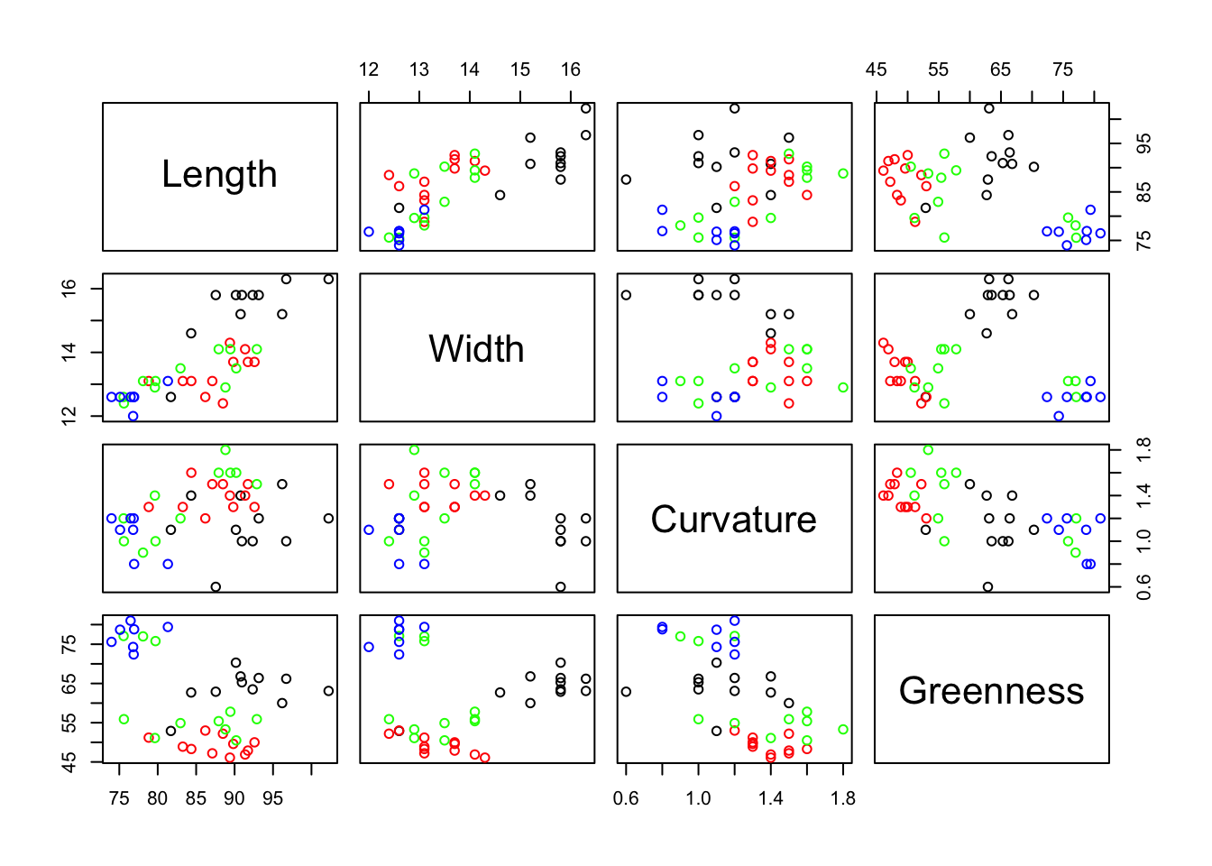
$ Days : int 36 100 67 86 127 114 111 116 128 115 ...Before applying any formal statistical analysis is always convenient to explore the data by computing some basic statistics and graphical representations. This gives you a first insight into the data and facilitates the detection of possible errors, outliers, trends, patterns, etc. A scatterplot matrix provides a helpful overview of the data, but of course it is not practical when the number of variables is large. The following line shows it for the numerical variables in the air pollution data set (columns 3 to 9).
The single scatterplot of Temp against Manuf suggests an outlier (the State with the very large value for Manuf). However, the Pop by Manuf scatterplot, and several others, show that although this State is extreme it is not really an outlier. There are some clearly non-normally distributed variables. You can check this out by plotting some histograms using hist of qq-plots using qqnorm).
Labels to identify individual points in a scatter diagram are often an essential aid to interpretation.
# “n” -  do not plot the symbols
plot(airpol$Temp, airpol$Manuf, type = "n")
# “text” adds labels to the current plot
text(airpol$Temp, airpol$Manuf, labels = airpol$Tn)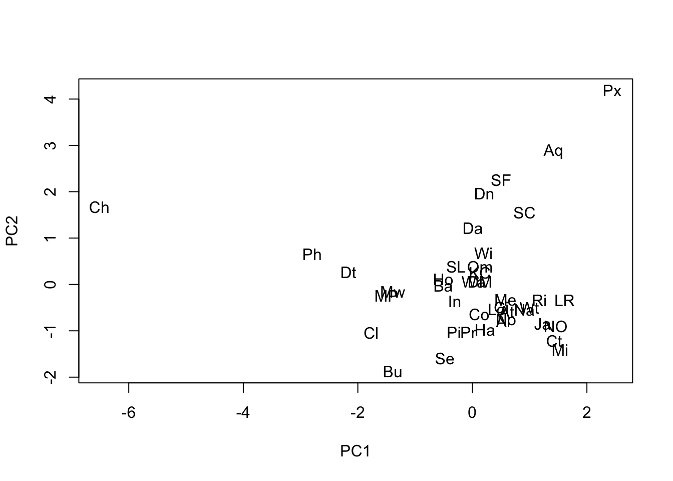
Chicago, a large city with a strong manufacturing base, was the potential outlier. The scatterplot matrix also reveals that there is one strong linear relationship, and possibly a second (Precip, Temp) though with a few States not fitting that pattern. Some non-normally distributed variables are also apparent.
Wind, despite being a discrete variable, appears approximately normally distributed.
As said, basic characteristics of the variables should be explored through summary statistics before proceeding to carry out any multivariate analysis. The most common being the sample mean and variance or standard deviation. The term sample refers to the fact that these measures are here computed from a real-world sample of data, in contrast with their population counterparts referring to the characteristics of the underlying random variables assumed to generate the observed data. When there is no possibility of confusion, they are simply called mean, variance, and so on. Given the \(i\)th variable (column) of the data set, the corresponding expressions are:
\[\begin{eqnarray} \mbox{Sample Mean }\overline{x}_i & = &\frac{1}{n}\,\sum_{k=1}^n x_{ki} \nonumber \\ \mbox{Sample variance }s^{2}_i & = & Var(x_i) = \frac{1}{n-1}\,\sum_{k=1}^n (x_{ki}-\overline{x}_i)^2 \nonumber \\ \mbox{Sample standard deviation }s_i & = & \sqrt{s^{2}_i} \nonumber \end{eqnarray}\]
Basic summary statistics can be obtained in R as follows:
      SO2              Temp           Manuf             Pop
 Min.   :  8.00   Min.   :43.50   Min.   :  35.0   Min.   :  71.0
 1st Qu.: 13.00   1st Qu.:50.60   1st Qu.: 181.0   1st Qu.: 299.0
 Median : 26.00   Median :54.60   Median : 347.0   Median : 515.0
 Mean   : 30.05   Mean   :55.76   Mean   : 463.1   Mean   : 608.6
 3rd Qu.: 35.00   3rd Qu.:59.30   3rd Qu.: 462.0   3rd Qu.: 717.0
 Max.   :110.00   Max.   :75.50   Max.   :3344.0   Max.   :3369.0
      Wind            Precip           Days
 Min.   : 6.000   Min.   : 7.05   Min.   : 36.0
 1st Qu.: 8.700   1st Qu.:30.96   1st Qu.:103.0
 Median : 9.300   Median :38.74   Median :115.0
 Mean   : 9.444   Mean   :36.77   Mean   :113.9
 3rd Qu.:10.600   3rd Qu.:43.11   3rd Qu.:128.0
Max. :12.700 Max. :59.80 Max. :166.0 SO2 Temp Manuf Pop Wind Precip Days
23.472272 7.227716 563.473948 579.113023 1.428644 11.771550 26.506419 We can notice that the scale and ranges of variation of the variables are very heterogeneous. With multivariate data we derive another fundamental summary statistic, the covariance matrix between every pair of variables.
\[\begin{eqnarray} \mbox{Sample covariance }s_{ij} & = & Cov(x_i,x_j) = \frac{1}{n-1}\,\sum_{k=1}^n(x_{ki}-\overline{x}_i)(x_{kj}-\overline{x}_j) \nonumber \end{eqnarray}\]
If the variable \(x_i\) is generally above its mean value whenever \(x_j\) is above its mean value then the covariance between them will be positive. If \(x_i\) is generally below its mean value whenever \(x_j\) is above its mean value then the covariance between them will be negative. The complete set of covariances for a set of variables is presented as a matrix.
          SO2   Temp  Manuf    Pop   Wind  Precip   Days
SO2     550.9  -73.6   8528   6712   3.18   15.00  229.9
Temp    -73.6   52.2   -774   -262  -3.61   32.86  -82.4
Manuf  8527.7 -774.0 317503 311719 191.55 -215.02 1969.0
Pop    6712.0 -262.3 311719 335372 175.93 -178.05  646.0
Wind      3.2   -3.6    192    176   2.04   -0.22    6.2
Precip   15.0   32.9   -215   -178  -0.22  138.57  154.8
Days    229.9  -82.4   1969    646   6.21  154.79  702.6
Notice that this matrix is symmetric, that is \(s_{ij}=s_{ji}\), and that the diagonal elements are the variances. Although covariance matrices play an important role in formal statistics, in practical data analysis they are not always easy to interpret and have the disadvantage that they are scale dependent. For example, multiply SO2 by 10 and all its covariances will increase by 10.
One of the most common scaling is to divide each variate by its own standard deviation. This forces every variate to have the same standard deviation, namely 1. In terms of variability all the variates are now on the same scale. A further consequence of this scaling is that the covariance matrix of the scaled variables is the so-called correlation matrix of the original variables.
\[\mathbf R = \left( \begin{array}{ccccc} 1 & r_{12} & . & . & r_{1p}\\ r_{21} & 1 & r_{23} & . & r_{2p} \\ . & . & . & . & . \\ . & . & . & . & . \\ r_{p1} & r_{p2} & r_{p3} & . & 1 \end{array} \right),\]
where the pairwise correlations are computed from the covariances and standard deviations as \(r_{ij}=\frac{s_{ij}}{s_is_j}\). The correlation matrix plays a fundamental role in multivariate data analysis. Correlation coefficients measure the extent to which two variables are linearly related. For example, the correlation between Pop and Manuf is 0.955 and between Precip and Temp is 0.386.
          SO2   Temp  Manuf    Pop   Wind Precip   Days
SO2     1.000 -0.434  0.645  0.494  0.095  0.054  0.370
Temp   -0.434  1.000 -0.190 -0.063 -0.350  0.386 -0.430
Manuf   0.645 -0.190  1.000  0.955  0.238 -0.032  0.132
Pop     0.494 -0.063  0.955  1.000  0.213 -0.026  0.042
Wind    0.095 -0.350  0.238  0.213  1.000 -0.013  0.164
Precip  0.054  0.386 -0.032 -0.026 -0.013  1.000  0.496
Days    0.370 -0.430  0.132  0.042  0.164  0.496  1.000
As several of the variables seem not be symmetrically distributed it is worth deriving the coefficient of skewness. This is estimated for a variable by the formula
\[g=\frac{1}{n}\sum_{k=1}^{n}(x_k-\overline{x})^3\frac{1}{s^3}\]
The following code creates this formula in R:
If applied to each numerical variable in the air pollution data we obtain
    SO2    Temp   Manuf     Pop    Wind  Precip    Days
 1.5841  0.8230  3.4846  2.9413  0.0027 -0.6925 -0.5501
These values quantify what the histograms show. For example, Manuf is very positively skewed but Precip and Days have a slight negative skew (tail of the histogram to the left).
1.3 Multivariate normal distribution
Much of univariate statistical theory depends on the variable of interest having a normal probability distribution. We write \(x\) ~ \(N(\mu,\sigma^2)\), where \(\mu\) and \(\sigma^2\) are the (population) mean and variance of the distribution of \(x\). These two parameters define the distribution completely. Many univariate methods are robust to modest departures from normality which is why often we need assurance that our data are at least approximately normally distributed.
There is a set of multivariate statistical methods which similarly depend on the variables of interest jointly having a multivariate normal distribution. If we have p variables \(x_1,\ldots,x_p\), we write these as a column vector \(\textbf{x}\) and say that \(\textbf{x}\) ~ \(N(\mu,\Sigma)\), where \(\mu\) is the column vector of (population) means and \(\Sigma\) is the (population) covariance matrix.
\[\mathbf{x} = \left( \begin{array}{c}x_{1} \\x_{2} \\ \vdots \\x_{p} \end{array} \right), \mu = \left( \begin{array}{c}\mu_{1} \\\mu_{2} \\ \vdots \\\mu_{p} \end{array} \right) \text{, and } \, \mbox{$\Sigma$} = \left( \begin{array}{ccccc} \sigma_{11} & \sigma_{12} & . & . & \sigma_{1p}\\ \sigma_{21} & \sigma_{22} & \sigma_{23} & . & \sigma_{2p} \\ . & . & . & . & . \\ . & . & . & . & . \\ \sigma_{p1} & \sigma_{p2} & \sigma_{p3} & . & \sigma_{pp} \end{array} \right)\]
When \(\textbf{x}\) has a multivariate normal distribution, each of the individual \(x_i\) has a univariate normal distribution. The manner in which the \(x_i\) are related to each other is described by the covariance matrix. The covariance matrix \(\Sigma\) is of theoretical interest, however the (population) correlation matrix \(\rho\) can be conceptually more useful.
\[ \left( \begin{array}{ccccc} 1 & \rho_{12} & . & . & \rho_{1p}\\ \rho_{21} & 1 & \rho_{23} & . & \rho_{2p} \\ . & . & . & . & . \\ . & . & . & . & . \\ \rho_{p1} & \rho_{p2} & \rho_{p3} & . & 1 \end{array} \right)\]
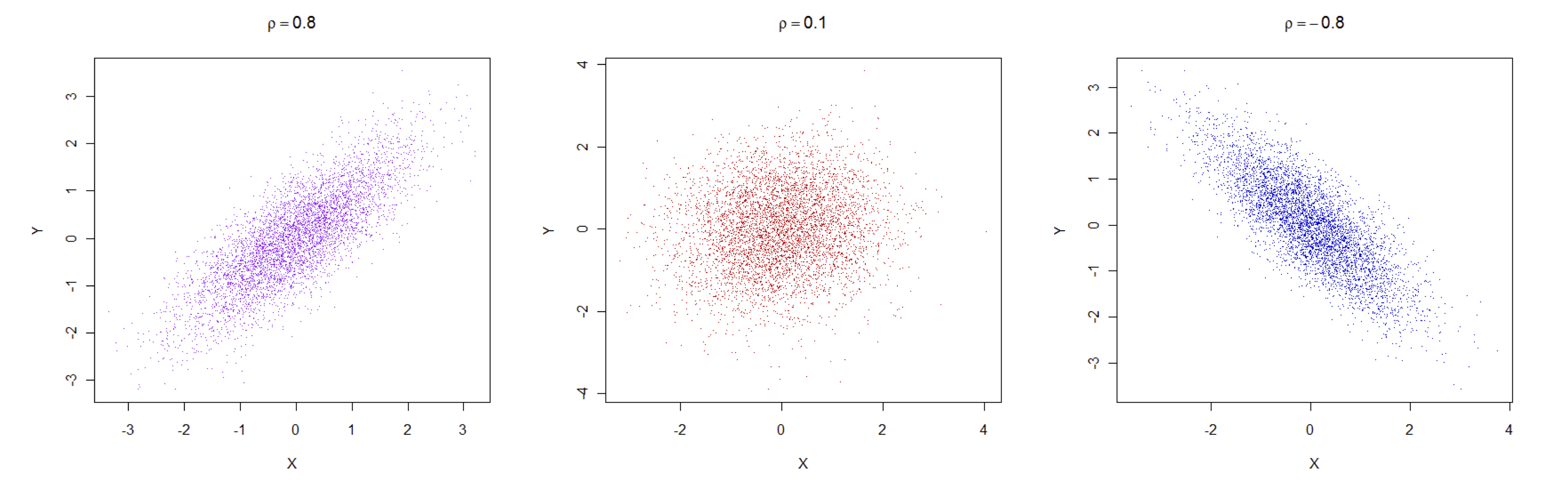
Covariances and correlations are closely linked as shown above: \(\rho{ij}=\sigma_{ij}/\sigma_{i}.\sigma_{j}\). In practice, correlations are more interpretable as they are unaffected by rescaling the variables, e.g. from cm. to mm., and the are defined in the interval \([-1,1]\), with \(-1\) meaning perfect negative correlation, \(1\) perfect positive correlation and \(0\) no correlation. The following figure shows exemplary cases of clouds of data points associated with correlations of 0.8, \(0.1\) and \(-0.8\).
1.4 Exercises
NIR data. Use a scatterplot matrix to see whether there is any relationship between protein, moisture and the first 10 wavelengths. How would you describe the relationships among the wavelengths? Derive the correlation matrix for protein, moisture and the first 10 wavelengths and use it to strengthen your conclusions based on the plots only. Use boxplots to get an overview of all the wavelengths, how their mean values and variation change across the NIR spectrum, i.e. as you move from the first to the last wavelength.
SOUP data. Use a scatter plot matrix to get an overview of the data. Look for a relationship between Tomato Flavour and Tomato Odour. Are there other similar relationships? Derive the summary statistics for these variables, i.e. means, standard deviations, minimums and maximums. Also look at the correlation matrix for all the variables. It should confirm what you saw in the scatterplot matrix graph.
RIME ICE data. Derive the mean, standard deviation and coefficient of skewness for the 14 elements. Are any of these 14 elements correlated with each other? Generate the scatterplot matrix for the elements and confirm that the most skewed elements in the plots have the largest (positive or negative) skewness coefficients. Use histograms to see whether any element is approximately normally distributed. Are the means and variances of any of the elements affected by whether they face North or South? For this last question you will need R statements of the form
tapply(element,ns,mean).