Chapter 11 Additive models
11.1 Introduction
We have already met smooth splines in the context of a single \(X\) variable, where we fit a smooth curve through the data points. We now extend that procedure to several \(X\) variables. For multiple regression we had
\[Y = b_0 + b_1X_1 + \ldots + b_pX_p + \epsilon\] Additive models instead consider smooth splines \(f\) for the explanatory variables
\[Y = b_0 + b_1f_1(X_1) + \ldots + b_pf_p(X_p) + \epsilon\] This provides a great flexibility to fit non-linear relationships between explanatory and response variables.
11.2 GAM analysis of the ozone data set
The package mgcv, accompanying the book Generalized Additive Models by Simon R. Wood, is the main reference to fit additive models in R. We will use it along with the ozone data set from the package faraway.
The ozone data are from a study in the Los Angeles Basin in 1976 to examine the relationship between ozone (\(O_3\)) and other meteorological variables. We will use only temperature (temp), inversion base height (ibh) and inversion top temperature (ibt).
'data.frame':   330 obs. of  10 variables:
 $ O3      : num  3 5 5 6 4 4 6 7 4 6 ...
 $ vh      : num  5710 5700 5760 5720 5790 5790 5700 5700 5770 5720 ...
 $ wind    : num  4 3 3 4 6 3 3 3 8 3 ...
 $ humidity: num  28 37 51 69 19 25 73 59 27 44 ...
 $ temp    : num  40 45 54 35 45 55 41 44 54 51 ...
 $ ibh     : num  2693 590 1450 1568 2631 ...
 $ dpg     : num  -25 -24 25 15 -33 -28 23 -2 -19 9 ...
 $ ibt     : num  87 128 139 121 123 182 114 91 92 173 ...
 $ vis     : num  250 100 60 60 100 250 120 120 120 150 ...
 $ doy     : num  33 34 35 36 37 38 39 40 41 42 ...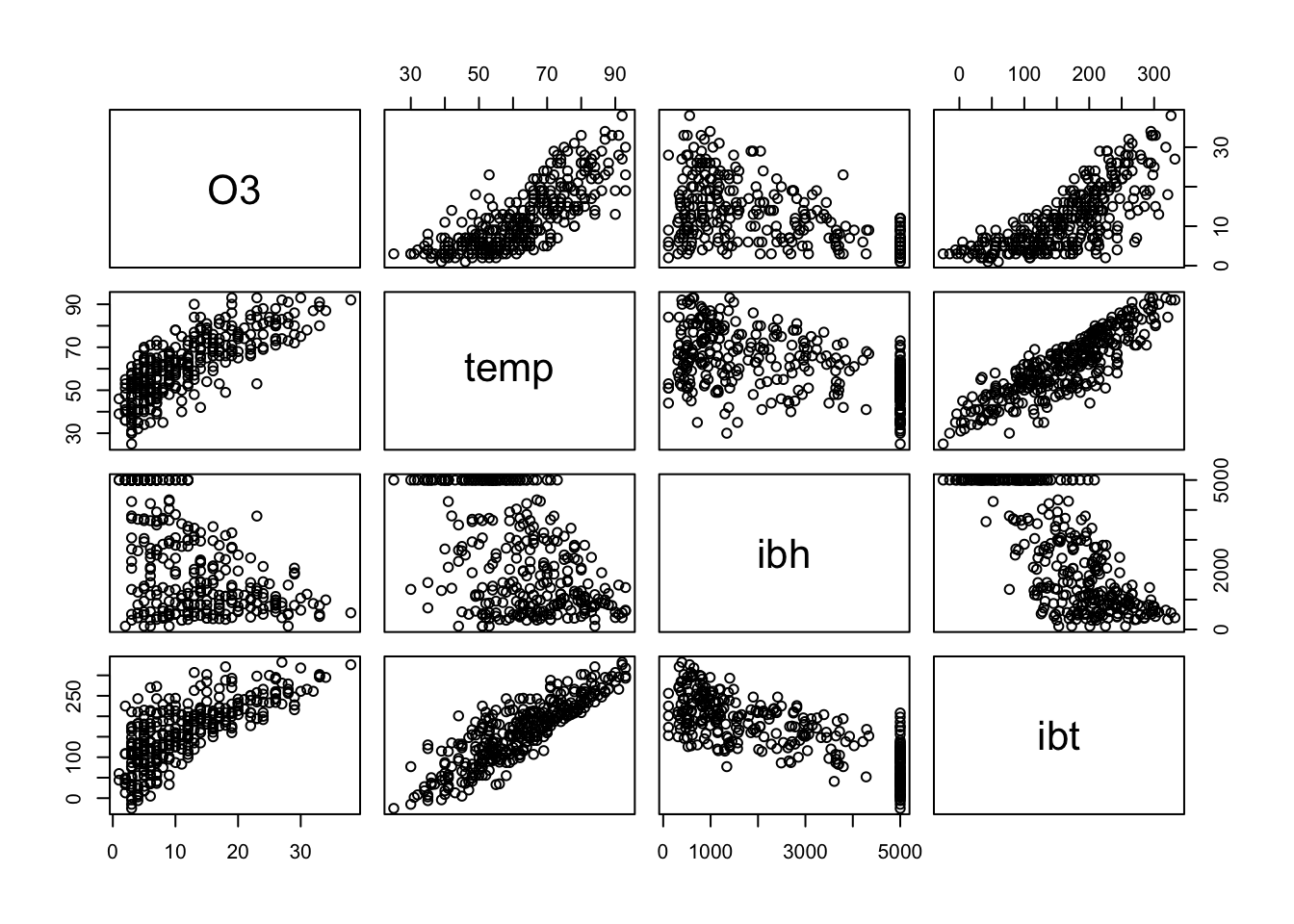
The pairs plot shows \(O_3\) responding non-linearly to temp and ibt, but we fit a simple linear model as a starting point.
Call:
lm(formula = O3 ~ temp + ibh + ibt, data = ozone)

Residuals:
     Min       1Q   Median       3Q      Max
-11.3224  -3.1913  -0.2591   2.9635  13.2860

Coefficients:
              Estimate Std. Error t value Pr(>|t|)
(Intercept) -7.7279822  1.6216623  -4.765 2.84e-06 ***
temp         0.3804408  0.0401582   9.474  < 2e-16 ***
ibh         -0.0011862  0.0002567  -4.621 5.52e-06 ***
ibt         -0.0058215  0.0101793  -0.572    0.568
---
Signif. codes:  0 '***' 0.001 '**' 0.01 '*' 0.05 '.' 0.1 ' ' 1

Residual standard error: 4.748 on 326 degrees of freedom
Multiple R-squared:  0.652, Adjusted R-squared:  0.6488
F-statistic: 203.6 on 3 and 326 DF,  p-value: < 2.2e-16
# Copy of current graphic parameters
oldpar <- par()
# Modify them to do a 2x2 matrix of graphs
par(oma = c(0, 0, 0, 0), mfrow=c(2, 2))
plot(m.olm)
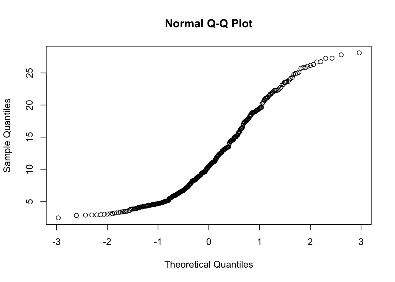
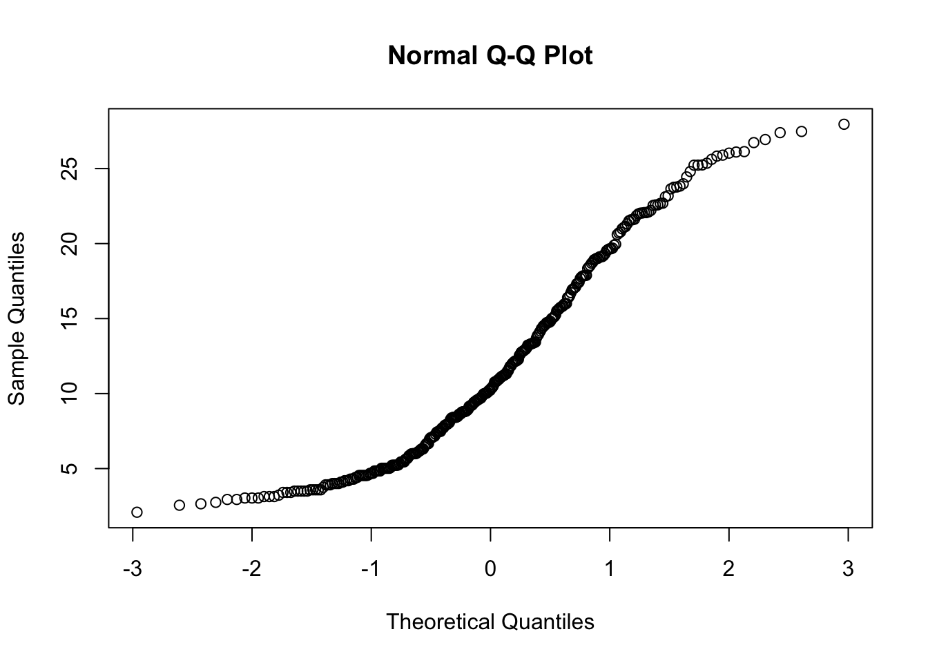
The residuals-versus-fitted plot indicates a problem of increasing variance as the mean of \(O_3\) increases and the q-q plot has a problem in its upper tail. We need to try something else.
In the following we use the function gam of the package mgcv to fit a generalised additive model (GAM) assuming a Gaussian response variable.
# install.packages("mgcv")
library(mgcv)
m.am <- gam(O3 ~ s(temp) + s(ibh) + s(ibt), data=ozone)
summary(m.am)
Family: gaussian
Link function: identity
Formula:
O3 ~ s(temp) + s(ibh) + s(ibt)
Parametric coefficients:
Estimate Std. Error t value Pr(>|t|)
(Intercept) 11.7758 0.2382 49.44 <2e-16 ***
---
Signif. codes: 0 '***' 0.001 '**' 0.01 '*' 0.05 '.' 0.1 ' ' 1
Approximate significance of smooth terms:
edf Ref.df F p-value
s(temp) 3.386 4.259 20.681 < 2e-16 ***
s(ibh) 4.174 5.076 7.338 1.74e-06 ***
s(ibt) 2.112 2.731 1.400 0.214
---
Signif. codes: 0 '***' 0.001 '**' 0.01 '*' 0.05 '.' 0.1 ' ' 1
R-sq.(adj) = 0.708 Deviance explained = 71.7%
GCV = 19.346 Scale est. = 18.72 n = 330This has done a little better than the ordinary linear model judging by the adjusted \(R^2\), but has used more degrees of freedom (edf in the R output). Again ibt seems not to affect \(O_3\). Note that gam has automatically determined the amount of smoothing. This is done by minimizing a cross-validation measure, the GCV score.
We can see the shape of the fitted smooth functions easily.
# Copy of current graphic parameters
oldpar <- par()
# Modify them to do a 2x2 matrix of graphs
par(oma = c(0, 0, 0, 0), mfrow=c(2, 2))
plot(m.am)
# Revert to original settings
par(oldpar)
These results suggest that the effect of ibt on \(O_3\) is minimal, that ibh has more effect but is highly variable and that temp has a strong positive link with \(O_3\) but that it might get stronger above 60 degrees.
The diagnostic plots have improved a little with respect to the linear model but not enough.
Next we drop ibt because it was not significant.
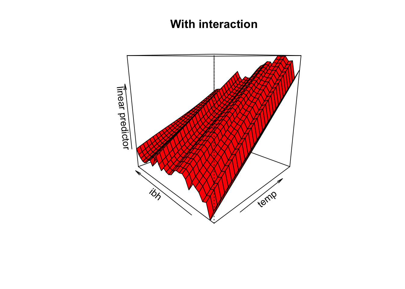
We also try a possible interaction between temp and ibh,
and note that the adjusted \(R^2\) has hardly changed from the model without the interaction term. It is easy to visualise the predictions from the model with interaction using vis.gam.
We can compare more formally models m.amint and m.am2 (with and without interaction) to confirm our conclusion that there is no need to allow for interaction.
Analysis of Deviance Table

Model 1: O3 ~ s(temp) + s(ibh)
Model 2: O3 ~ s(temp, ibh)
  Resid. Df Resid. Dev     Df Deviance      F Pr(>F)
1    319.11     6054.0
2    301.92     5896.1 17.197   157.91 0.4755 0.9636
The \(F\)-test suggests that the models are actually statistically comparable and it is not worth including the interaction term.
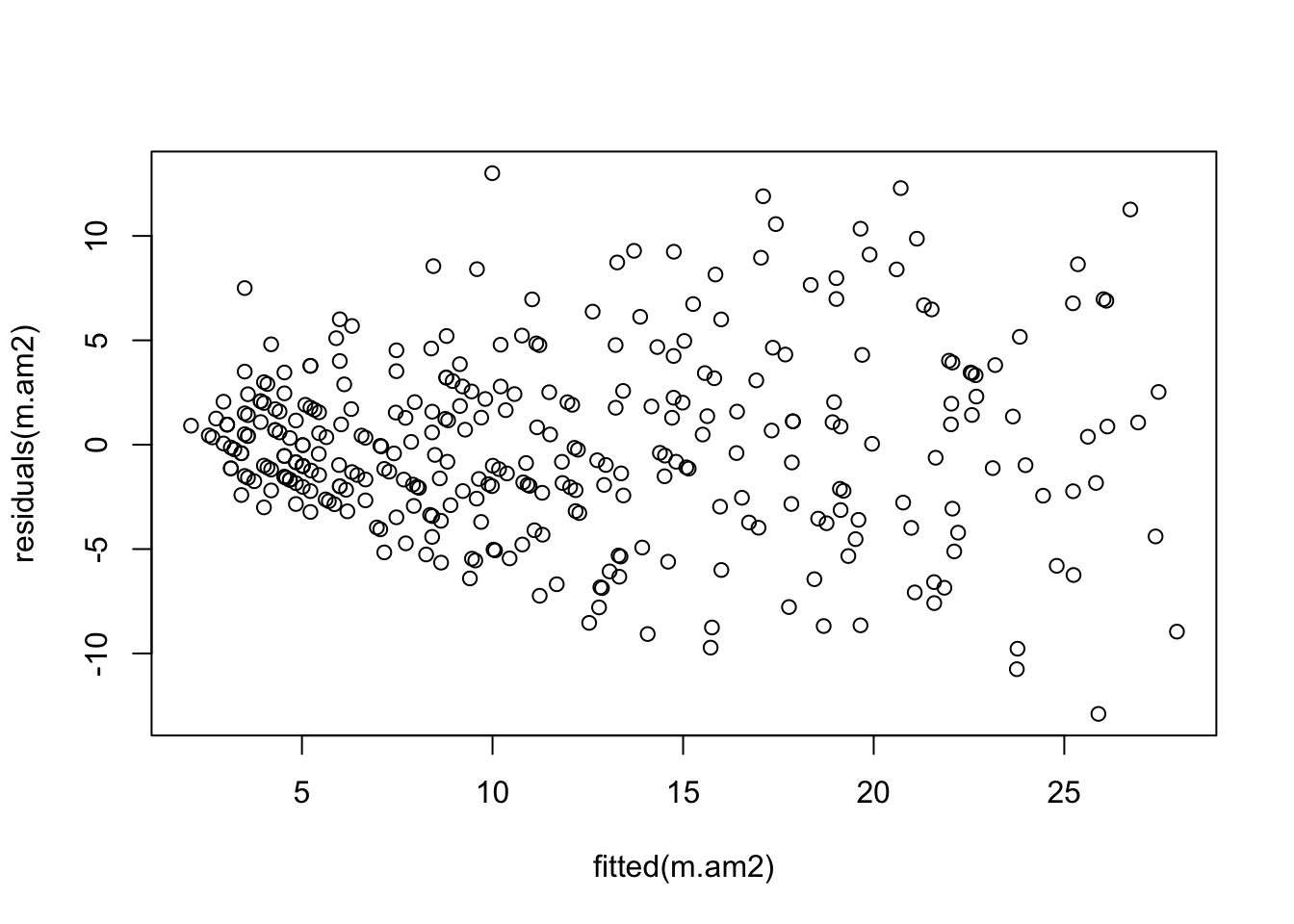
The diagnostic plots for model m.am2 still leave room for improvement.
While smooth functions do not provide mathematical formulae or parameters by which we can characterise a process, they are sometimes used as a first step in determining an appropriate parametric model.
Alternatively, the plots for model m.am hint that both temp and ibh might affect \(O_3\) in a ‘broken stick’ manner. The response of \(O_3\) might be a function of two different straight lines with the break point at \(temp=60\); similarly for ibh with a break point at \(ibh=1000\). We can explore this possibility considering the following linear model.
rhs <- function(x,c) ifelse(x>c,x-c,0)
lhs <- function(x,c) ifelse(x<c,c-x,0)
m.olm2 <-
  lm(O3 ~ rhs(temp, 60) +
          lhs(temp, 60) +
          rhs(ibh, 1000) +
          lhs(ibh, 1000),
          data = ozone)
summary(m.olm2)
Call:
lm(formula = O3 ~ rhs(temp, 60) + lhs(temp, 60) + rhs(ibh, 1000) +
    lhs(ibh, 1000), data = ozone)

Residuals:
     Min       1Q   Median       3Q      Max
-13.2042  -2.6307  -0.2887   2.3179  12.6720

Coefficients:
                 Estimate Std. Error t value Pr(>|t|)
(Intercept)    11.6038321  0.6226512  18.636  < 2e-16 ***
rhs(temp, 60)   0.5364407  0.0331849  16.165  < 2e-16 ***
lhs(temp, 60)  -0.1161735  0.0378660  -3.068  0.00234 **
rhs(ibh, 1000) -0.0014859  0.0001985  -7.486 6.72e-13 ***
lhs(ibh, 1000) -0.0035544  0.0013138  -2.705  0.00718 **
---
Signif. codes:  0 '***' 0.001 '**' 0.01 '*' 0.05 '.' 0.1 ' ' 1

Residual standard error: 4.342 on 325 degrees of freedom
Multiple R-squared:  0.7098,    Adjusted R-squared:  0.7062
F-statistic: 198.7 on 4 and 325 DF,  p-value: < 2.2e-16
Adjusted \(R^2\), residual standard error and diagnostic plots (not shown) all indicate the same degree of goodness of fit and the same problems as the m.am2 model. What we have gained is an explicit model with parameters we can use to compare directly with other data sets.
To see the weakness of the m.olm2 model more clearly we plot its fitted values against the actual \(O_3\) values.
with(ozone, plot(O3,fitted(m.olm2), ylim=c(0,40), xlim=c(0,40),
                 main="Actual vs fitted, broken stick") )
abline(a=0,b=1)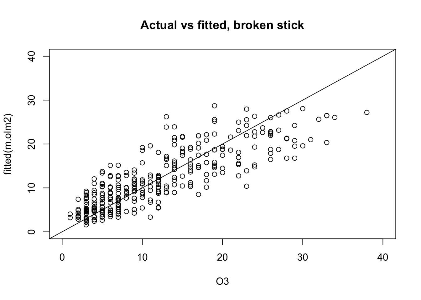
Using the ozone data set we have illustrated the use of additive models with a Gaussian response variable. However, sticking with the package mgcv and the same function gam we can easily extend this to generalized additive models (GAMs) through the family argument. This allows to use smooth functions to fit models with no Gaussian responses in a form equivalent to fitting generalised linear models using glm as we discussed before.
11.3 Exercises
One of the weaknesses with all of the ozone additive models we have tried is the increasing variance in the residuals as the mean value of \(O_3\) increased. Try modelling \(O_3\) as following a Gamma distribution with identity link instead of the default Gaussian distribution. This will allow for increasing variance as \(O_3\) increases. Comment the results in comparison with the previous models fitted.
With the savings data is there any merit in using smooth functions rather than linear functions to predict sr?